25. Basics of DCE MRI
25.1. DCE MRI experiment and analysis
This section summarizes the information about the T1-weighted dynamic contrast-enhanced MRI (DCE MRI) MRI and issues related to the quantification of contrast concentration and tissue parameters from DCE MRI data.
A typical DCE MRI experiment (for quantitative model analysis) involves:
Human subjects imaged at 1.5 T or 3.0 T,
Bolus injection of Gd-based contrast agent (GBCA) into a peripheral vein,
Serial images acquired using T1-weighted gradient-echo (GRE) sequence with temporal resolution of a few seconds (15 s or less),
Images acquired in coronal, oblique coronal, or axial plane,
Blood signal sampled in a vessel feeding the tissue of interest to determine the arterial input function (AIF) driving a compartmental model describing the tissue,
Tissue and blood signal converted to gadolinium (Gd) concentration,
Model fitting of tissue concentration performed to derive tissue parameters.
In the first approximation, all complexities are ignored (non-uniformity, artifacts, high field imaging, parallel imaging, animal imaging, etc.).
25.2. Contrast agents: Safety, dose, concentration, and volume
25.2.1. Contrast agent safety
The FDA-approved gadolinium-based contrast agents (GBCA) currently include: Dotarem (Clariscan), Eovist, Gadavist (Gadovist), Magnevist, MultiHance, Omniscan, Optimark, and ProHance. Among these, Eovist is used to detect and characterize liver lesions. The other GBCA may be used for DCE MRI in the brain and body.
Since the late 1990x, GBCA have been found to increase the risk of nephrogenic systemic fibrosis (NSF), a rare, but serious, condition in patients with kidney dysfunction (FDA 2010). The risk of NSF was the highest for linear GBCA (such as Magnevist, Omniscan, and Optimark) and in patients with estimated glomerular filtration rate GFR <30 mL/min/1.73m2. As a result, in the European Union, since 2017 the use of linear GBCA has been suspended, except in liver imaging (European Medicines Agency 2017).
Since the adoption of safety measures (such as using predominantly macrocyclic GBCA and screening patients with severe, chronic kidney disease (CKD) or acute kidney injury (AKI)), new cases of unconfounded NSF have been nearly eliminated.
Subsequently, it has been determined that gadolinium from GBCA is retained in the brain, liver, bone, and skin (Mathur 2020 PMID: 31809230; Marks 2021 PMID: 33868652).
The retention of gadolinium is higher with Omniscan and Optimark than after Eovist, Magnevist, or MultiHance. The retention is the least after Dotarem, Gadavist, or ProHance.
The updated FDA recommendations (FDA 2018) advise considering the retention characteristics of each agent for patients at risk and using GBCA judiciously, especially for repeated examinations. Although the deposition of gadolinium in the brain has not been linked to any adverse effects on health, risk-to-benefit ratio of GBCA use is advised in each case.
25.2.2. Injected dose
The dose of gadolinium (in millimoles, mmol) administered to the patient may be:
A fixed amount, constant for all patients in the cohort, or, more commonly,
An amount proportional to the patient’s weight (typically 0.1-0.2 mmol/kg). Thus, a patient weighing 80 kg and dosed at 0.1 mmol/kg will receive 8 mmol of gadolinium.
For repeat studies (such as the evaluation of response to treatment), it is important that the dose be determined the same way for the baseline and the follow-up examinations.
25.2.3. Contrast agent concentration
Contrast agents are formulated as solutions with different concentrations of gadolinium (Table 25.1).
Contrast Agent |
Concentration (mmol/mL) |
|---|---|
Magnevist, ProHance, Omniscan, MultiHance, Dotarem/Clariscan |
0.50 |
Gadavist (US) (Gadovist elsewhere) |
1.00 |
Eovist |
0.25 |
The FDA label format varies and may list: concentration in mg/mL, mmol/mL, or mmol/L, molar mass, recommended dose per weight for different applications, and other parameters.
25.2.4. Injected volume of contrast agent
The injected volume is equal to the dose of Gd (mmol) divided by concentration (mmol/mL). Thus, the patient receiving 8 mmol of Gd would need 16 mL of MultiHance, but only 8 mL of Gadavist.
25.3. Conversion of MRI signal to contrast concentration
25.3.1. Fast exchange limit
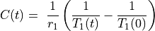
DCE MRI data are often analyzed assuming fast water exchange, when water protons in tissue move across tissue compartments much faster than they interact with the contrast agent. The tissue is then described by a single, uniform relaxation rate R1 (or relaxation time T1, so that R1=1/T1) and the change in R1 is proportional to the concentration of Gd contrast:
(25.1)
where:
– concentration of Gd (units: mmol/L = mM)
– longitudinal relaxivity of the contrast agent (L/(mmol x s) = mM-1 s-1)
– pre-contrast longitudinal relaxation time of blood or tissue (s)
– post-contrast longitudinal relaxation time of blood or tissue (s).
25.3.2. Concentration units
The concentration units (for tissue or blood) are customarily mmol/L = mM. In the US, the preferred notation for liter and milliliter is L and mL, respectively (NIST SP330 2019, p. iii and p. 25, Table 8). However, lower case l and ml are often used as well (US Metric Association).
25.3.3. Relaxivity of the contrast agent
Relaxivity of the contrast agent is dependent on magnetic field strength, temperature, and medium (e.g., water, plasma, or whole blood) and is usually obtained from manufacturer’s data and literature. For example, at 3 T in human plasma, the relaxivity of ProHance (gadoteridol) is r1=3.28 mM-1 s-1 and Gadavist (gadobutrol) r1= 4.97 mM-1 s-1.
25.3.4. Pre-contrast T10 in tissues and blood
25.3.4.1. Tissue T10
Pre-contrast T10 in tissue may be measured individually (and quantified via ROI- or voxel-by-voxel fitting) or assigned a fixed value for a given tissue type and field strength. Examples of T10 measurements in various tissues include:
Abdomen 1.5T and 3T – de Bazelaire 2004 PMID: 14990831
Breast 1.5T and 3T – Rakow-Penner 2006 PMID: 16315211
Brain and body 3T (extensive collection of literature T10 and T20 values) – Zavala Bojorquez 2017 PMID: 27594531
Brain at 1.5T, 3T, 7T – Wright 2008 PMID: 18259791.
25.3.4.2. Blood T10
Pre-contrast blood T10 varies with the field strength, temperature, and blood oxygenation. Fixed literature values of blood T10 are often used DCE MRI analysis (see examples in Table 25.2).
Reference/Experiment |
Measured in |
Field |
T10 (ms) |
|---|---|---|---|
Lu et al. 2004. PMID 15334591 Flow phantom 37°C |
|||
Arterial blood |
3T |
1664 |
|
Venous blood |
3T |
1584 |
|
Zhang et al. 2013. PMID 23172845 Healthy volunteers (sagittal sinus) |
|||
Venous blood |
1.5T |
1480 |
|
Venous blood |
3T |
1649 |
|
Venous blood |
7T |
2087 |
|
Shimada et al. 2012. PMID 23269013 Healthy volunteers (abdominal aorta, jugular vein) |
|||
Arterial blood |
3T |
1779 |
|
Venous blood |
3T |
1694 |
|
Vatnehol et al. 2019. PMID 30604145 Healthy volunteers (portal vein) |
|||
Venous blood |
3T |
1733 |
As noted by Zhang et al. (Zhang 2013 PMID: 23172845), “At 1.5 T, arterial and venous blood T1 values are virtually the same, whereas arterial blood T1 is 79 ms higher than venous blood T1 at 3 T and 330 ms at 4.7 T.”
Additionally, in vitro T10 of blood and plasma are often reported in studies of contrast agent relaxivity (Shen 2015 PMID: 25658049; Rohrer 2005 PMID: 16230904).
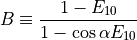
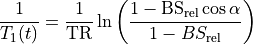
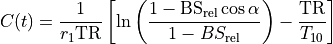
25.3.5. Signal to concentration conversion with gradient echo signal expression
MRI signal can be related to blood or tissue relaxation rate R1=1/T1 using the Spoiled Gradient Recalled (SPGR) echo signal expression:
(25.2)
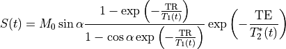
where TR is the repetition time and  is the flip angle.
M0 is the equilibrium magnetization (for
is the flip angle.
M0 is the equilibrium magnetization (for  and TR>>T1(0), which accounts for the spin density and receiver gain.
At short TE (TE<<T2*), the T2* effect can be ignored (Schabel & Parker 2008 PMID: 18421121):
(25.3)
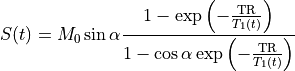
At high Gd concentrations, the assumption of TE<<T2* may no longer be valid. However, correcting for T2* has its own challenges.
The concentration C(t) may be obtained by solving Eq. (25.3) for 1/T1(t) and plugging it into Eq. (25.1). The expressions for C(t) and T1(t) are available in several forms, with slight differences in notation.

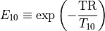
25.3.6. Linear approximation at low concentration
At low contrast concentrations (i.e., when the contrast does not alter
the spin density and T2* effects are negligible), the signal
in Eq. (25.3) (at  and TR/T1<<1)
is approximately linear with 1/T1
(Buckley & Parker in DCE MRI in Oncology 2005):
and TR/T1<<1)
is approximately linear with 1/T1
(Buckley & Parker in DCE MRI in Oncology 2005):
(25.6)
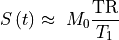
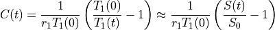
Then the concentration from Eq. (25.6) is approximately linearly related to the signal enhancement (Wake 2018 PMID: 29777820):
(25.7)
This approximation may be appropriate at low concentrations. However, it may not be optimal for converting the signal of blood in dynamic contrast-enhanced MRI with bolus injections of contrast, especially during the first-pass peak.