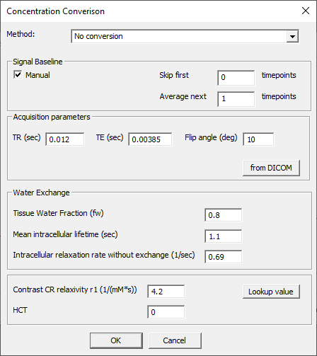
The signal-to-concentration conversion can be performed
Concentration Conversion dialog, available under
the Dynamic Analysis tab and through other commands
(Fig. 34.1).
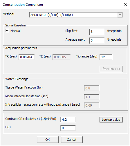
Fig. 34.1 Concentration Conversion dialog in its default state.
The Conversion dialog can be accessed via the following routes:
Dynamic Analysis > Convert TAC to Concentration.
This option is available with and without images loaded into FireVoxel.
The command launches browse-for-file dialog to select a the input text file,
in which the first two columns contain (1) time and (2) signal intensity values.
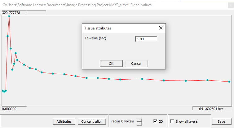
Once a compatible file has been selected, the signal values versus time
are displayed in a new panel (Signal values, Fig. 34.2).
The user can inspect the signal curve and set up the conversion using
the buttons at the bottom of this panel.
Attributes – Opens dialog for entering the precontrast T of tissue
of interest (in seconds) (see Attributes dialog Fig. 34.2).
Fig. 34.2 Concentration Conversion panel in its default state.
2. Calculate Parametric Map > Concentration (for AIF)
or Tissue Concentration (for tissue).
This option is available when the 4D dataset is recognized
as a dynamic contrast-enhanced MRI time series and the model requires
signal-to-concentration conversion (such as the Tofts model).
Clicking the Concentration buttons opens the Concentration Conversion
dialog for blood and tissue, respectively.
See Dynamic Analysis
and DCE MRI Model Analysis.
3. Cardiac Output Measurement and Correction > Concentration.
This command opens a dialog panel enables the user to load and display
signal intensity data and convert it to concentration by clicking
Concentration button, which opens Concentration Conversion dialog.
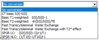
A dropdown menu with a selection of conversion scenarios
(Fig. 34.3).
The first entry (Signal values, default, no conversion)
applies to both CT and MRI. The second method (CT basic)
is for converting CT data, and the subsequent methods are
for MRI data.
Fig. 34.3 Conversion methods in Concentration Conversion panel.
Signal values – Default – No conversion, retains original signal intensity values.
CT basic S(t)–S(0) – Returns CT HU level corrected for baseline S(0).
The baseline can be determined automatically or manually (see Signal Baseline).
Basic T1-weighted: S(t)/S(0)–1 – Returns signal enhancement for T1-weighted MRI.
The method assumes linear relationship between signal enhancement and contrast
concentration. The effect of tissue precontrast T10 is ignored.
Basic T2-weighted: –ln(S(t)/S(0))/TE – Returns R2 values from T2-weighted MRI,
with signal given by: S(t)=S(0)*exp(-TE/T2), where TE is the echo time (see Acquisition).
Fast Transcytolemmal Water Exchange – UNDER DEVELOPMENT. Returns contrast
concentration (in mmol/L) for T1-weighted MRI signal. The conversion is done
using the shutter speed water exchange model for TE<<T2* in fast exchange regime (FXR)
(see Water Exchange).
Fast Transcytolemmal Water Exchange with T2* effect – UNDER DEVELOPMENT.
Returns contrast concentration (in mmol/L) for T1-weighted MRI signal with
the shutter speed model in FXR regime with accounting for T2* effect. REQUIRES TE?
Two Site Water Exchange – Returns contrast concentration (in mmol/L)
for T1-weighted MRI signal with the shutter speed model in two-site exchange
(2SX) regime for water molecules exchanging between intracellular and extracellular
compartments.
SPGR LC: (S(t)/S(0)–1)/r1/T10 – Returns contrast concentration (in mmol/L)
for T1-weighted MRI signal in fast exchange limit. The conversion is done with
linearized Spoiled Gradient Recalled Echo (SPGR) signal expression
(linear conversion, LC) (See Eq. (33.7)). Requires pre-contrast tissue
T10 (see Attributes) and relaxivity of contrast agent r1
to be selected in Contrast.
SPGR NLC: (1/T(t)–1/T10)/r1 – Returns contrast concentration (in mmol/L)
for T1-weighted MRI computed using SPGR signal equation
(nonlinear signal-to-concentration conversion, NLC) (See Eq. (33.5)).
Requires pre-contrast tissue T10 entered in Attributes.
This part enables the user to control how the baseline (pre-contrast)
signal S(0) is determined.
By default, the signal baseline is determined by averaging the data
points from the first data point to the contrast arrival time.
ADD DETAILS: HOW IS THE CONTRAST ARRIVAL TIME DETERMINED?
Alternatively, the user may select the baseline to be determined
manually (e.g., when the first data points are problematic).
Manual – Checkbox which, if checked, allows the user to specify
the baseline points manually using the following options:
Skip first [X] timepoints – Text box to enter the number of
time points Nskip to be excluded from baseline computation:
timepoints 1, 2…, Nskip will be ignored.
Average next [X] timepoints – Text box to enter the number
of timepoints Navg, to be used as the baseline:
signal at timepoints
Nskip+1, Nskip+2,…, Nskip+ Navg
will be averaged to determine the baseline.
Here the sequence parameters – repetition time (TR, seconds), echo time (TE, seconds),
and flip angle (FA, degrees) - required for the conversion can be entered
manually into the corresponding text boxes.
Only parameters required by the selected conversion Method can be entered;
the unused parameter(s) are grayed out and cannot be changed (Fig. 34.4).
The sequence parameters may be loaded directly from the DICOM header
when the user clicks from DICOM button.
This option is available only when DICOM images are open in the active document window,
and the conversion is performed for the ROIs in the same window.
This is the case, for example, when the Concentration Conversion panel is accessed
from Calculate Parametric Map, when the active document window contains
DICOM images as well as the IDIF ROI and the tissue ROI, which are used to compute
the model parameters.
Fig. 34.4 Concentration Conversion panel set up for nonlinear conversion
with a manual baseline, TR=2.84 ms, FA=12 deg.
This part specifies the parameters of the conversion using
the shutter speed water exchange model
(see Yankeelov et al. 2003. PMID:14648563,
Landis et al. 2000. PMID:11025512,
and critical discussion in Buckley 2019. PMID:30230007).
Tissue Water Fraction (fw) – Tissue volume fraction accessible
to mobile water solutes f_w (unitless; default, 0.8).
Mean intracellular lifetime (sec) – Mean lifetime of a water molecule
in intracellular compartment, (in seconds; default, 1.1 s).
Intracellular relaxation rate without exchange (1/sec) – Intracellular rate
constant without exchange, denoted (in inverse seconds; default, 0.69).
Text box labeled CR relaxivity r1 (1/(mM x s)) is for entering contrast agent
relaxivity value r1 (Fig. 34.4).
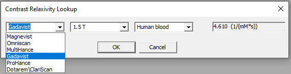
Lookup Value - Opens a sub-panel that allows the user
to select literature values of r1 relaxivity
for six currently approved contrast agents:
Magnevist, Omniscan, MultiHance, Gadavist, ProHance,
and Dotarem\Clariscan (Fig. 34.5).
The appropriate r1 value can be obtained using three drop-down menus to choose:
1) contrast agent, 2) field strength (1.5 T, 3 T, 7 T), and 3) medium
(human blood, human plasma, bovine blood, bovine plasma, canine blood,
canine plasma) matching the user’s experimental conditions.
Fig. 34.5 Lookup Value panel for selecting contrast agent relaxivity value
from literature
for the experimental conditions (contrast, field strength, and medium).
34.1.5.1. Literature values of relaxivity r1 (1/(mM s))
Text box for entering the value of hematocrit (HCT).
This is done to determine the concentration of contrast in plasma
instead of the whole blood by excluding the volume occupied by the blood cells:
Cplasma = Cwhole_blood / (1 – HCT).
By default, HCT=0 (no correction).
The user clicks OK on the Concentration Conversion panel.
The result is displayed as a plot of concentration (in mM) versus time,
if the command was accessed through Convert TAC to Concentration or
Cardiac Output Measurement and Correction.
The user can save the concentration as a text file by clicking Save
(or Save Original). The output file contains two columns: time
(as in the input data file) and concentration (in mM).
If the conversion was called via the Calculate Parametric Map dialog,
the concentration is not displayed.
 (in seconds; default, 1.1 s).
 (in inverse seconds; default, 0.69).