FireVoxel’s Nonuniformity tab provides access to several nonuniformity
correction methods for MR images. The user may choose the most
appropriate method based on the type of images, the severity of
nonuniformity artifact and resources available for image processing
(such as time and computing power).
Non-uniformity of image intensity is a common MRI artifact. It creates a
smooth variation of signal intensity across the image that is unrelated
to tissue properties. This artifact may be caused by the imperfections
of the imaging technique or the patient’s influence on the magnetic and
electric fields. Non-uniformity is often unnoticeable to a human
observer, but it may introduce errors into quantitative MRI methods,
such as segmentation, registration, and dynamic modeling. To minimize
these errors, it is often helpful to remove the non-uniformity artifact
before analyzing images.
A number of methods have been developed to minimize the nonuniformity
artifacts, including prospective and retrospective methods. Prospective
methods rely on additional sequences acquired during the MRI exam and
then used during processing for nonuniformity reduction. Retrospective
methods, such as the methods available in FireVoxel, estimate the
nonuniformities directly, without the need for additional acquisitions.
These methods assume that nonuniformity is multiplicative, which means
that the intensity of the acquired image at every point can be
represented as a product of the corrected intensity and a spatially
varying bias field (20.1):
FireVoxel offers three retrospective methods for non-uniformity
correction: the widely-used N3 method and its variant N4, as well as
FireVoxel’s original method, BiCal. The N3 method, for Non-parametric
Non-uniformity Normalization (Sled 1998, PMID:
9617910) is offered in the
streamlined local implementation (Tsui W, NYU School of Medicine, 2003).
The N4 method (Tustison 2010, PMID
20378467), a variant of
N3, is included as a plugin, N4BiasFieldCorrection.exe, in the FireVoxel
directory. The BiCal method (Mikheev A, Rusinek H, NYU School of Medicine,
2010) is a powerful method for challenging imaging situations, such as
abdominal, high field, and accelerated MRI.
The choice of method is usually motivated by a compromise between the
quality of correction and computational resources and time available.
Among these three methods, N3 is the fastest but the least powerful, and
BiCal is the slowest, but may be better suited for complex imaging
problems, such as high field imaging.
Additionally, N4 Explorer and BiCal Explorer enable parameter
optimization by running corrections with a grid of parameters. The tab
also contains options for measuring nonuniformity via coefficient of
variation (CV), coefficient of joint variation (CJV), and spillover for
two ROI layers.
The correction methods act on 3D or 4D images. For 4D images,
if the current image is not the first frame in the dynamic series,
FireVoxel shows a warning and asks the user whether to proceed or cancel
the correction. If the user chooses to proceed, only the current frame
will be corrected. No warning is shown for correction of the first image
in dynamic series, and only the first image is corrected.
Each of the three correction commands (N3, N4, and BiCal) opens a dialog
panel with adjustable options. The output includes the corrected image
or an option to create a bias field map. [N3 – checked checkbox Bias
Field creates only bias field, but no corrected image]. The corrected
images are placed in new layers named [active_layer]_N3 (or _N4 or
_BiCal). Bias field maps are placed in new layers named
[active_layer]_N3_BiasField.
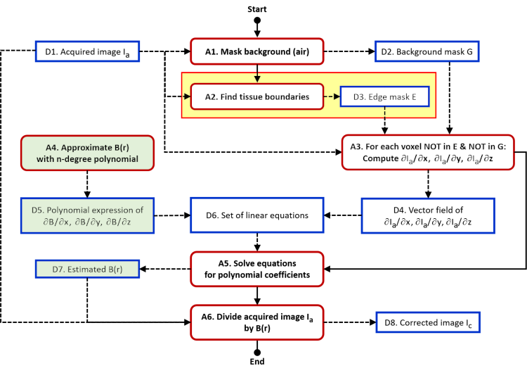
Below is a brief description of the algorithms for N3 and its
variant N4 methods (Fig. 20.1). N3, or Non-parametric
Non-uniformity Normalization, is the most commonly used non-uniformity
correction method. Both N3 and N4 methods operate in the log-transform space
of the image intensities and bias field. These methods deal with the
probability densities, or, for discrete images, intensity histograms.
The histogram of the logarithm of the bias field is assumed to be a
zero-centered Gaussian. Below is an overview of the internal steps of
the N3 and N4 algorithms.
First, the image background is masked. This initial step is followed by
an iterative block performed in the log-transform space of the image
intensities and bias field. The logarithmic transformation conveniently
changes the multiplication to addition, but may run into problems in
areas where signal intensity approaches zero, such as the air-filled
background regions. Masking the background helps to minimize these
potential issues. Within the iterative block, each iteration includes
three steps.
In Step 1, the bias field histogram is estimated so that the
corrected image is sharpened. This sharpening is achieved by applying
the Wiener deconvolution filter to the image intensity histogram. The
Wiener filter uses a Gaussian kernel with a full width at half maximum
(FWHM) selected by the user.
In Step 2, the new estimate of the bias field is smoothed by fitting
it with a three-dimensional B-spline field with a user-specified grid
size (given in millimeters). The size of the grid controls the degree
of smoothing. This grid size is typically about 200 millimeters for
images acquired with a body coil and smaller for images acquired with
localized surface coils.
In Step 3, the termination criterion is tested against a specified
threshold. In practice, the algorithm stops after a fixed number of
iterations specified by the user.
Once the iterations are completed, the bias field is extrapolated over
the entire field of view. Finally, the original image is divided by the
bias field to obtain the corrected image.
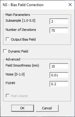
Selecting N3 on the Nonuniformity tab opens a parameter panel
(N3 – Bias Field Correction, Fig. 20.2), where the user can specify
the method parameters. The three key parameters, as described in the N3/N4
algorithm, are: Number of iterations (exit parameter in Step 3),
Field Smoothness (grid size in Step 2), and FWHM of the Gaussian
kernel (Step 1).
Additional parameters:
Subsample – ADD DETAILS
Dynamic Field (checkbox) – ADD DETAILS
Noise – ADD DETAILS
(Pad volume – currently disabled)
By default, the operation creates a corrected image in a newly added
layer. Checking Output Bias Field checkbox creates instead a new
layer with the bias field map.
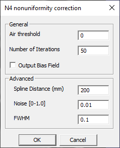
The N4 command opens a parameter panel (N4 nonuniformity correction,
Fig. 20.3)
with parameters of the N3/N4 algorithm: Number of Iterations, Spline
Distance (grid size, mm), and FWHM.
Background mask parameters (?):
Air threshold – ADD DETAILS
Noise – ADD DETAILS
By default, the output is the corrected image placed in a new layer.
Checking Output Bias Field creates instead a new layer with the bias
field map.
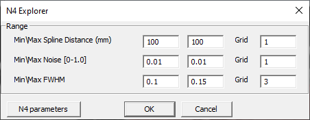
Enables optimization of N4 parameters. Requires a visible ROI
comprising multiple blobs scattered uniformly across the image.
If the document has no visible ROI, the command shows a warning.
Opens an N4 Explorer panel (Fig. 20.4) to test combinations
of values for three parameters: Spline Distance, Noise, and FVHM.
The parameters are sampled on a grid between the minimum and maximum values
at a set number of grid steps (Grid).
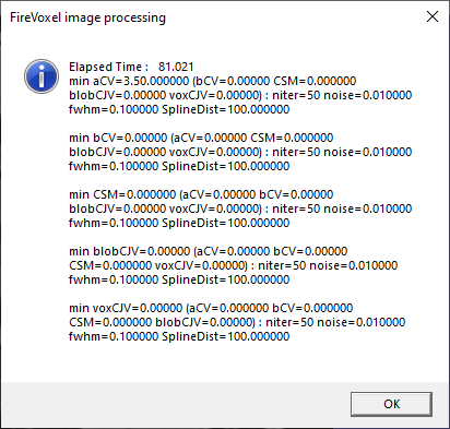
The results include coefficients aCV, bCV, CSM, blobCJV, voxCJV
(Fig. 20.5).
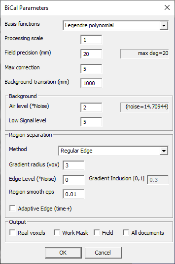
First, the background signal is removed from the acquired image to
create a background mask. The algorithm then detects sharp edges and
creates an edge mask, a key step in this method. The next three
action steps are performed in the log-transform space of the image
intensities and bias field, as in the N3 and N4 methods.
In the first of these three steps, the partial derivatives of the
image intensity are computed for each voxel of the body. The bias field
is estimated as a set of smooth polynomial functions and the partial
derivatives of the bias field are fitted directly to the partial
derivatives of the image signal intensity.
The resulting set of linear equations is solved to obtain the
polynomial coefficients that are used to estimate the bias field.
Finally, the acquired image is divided by the bias field to obtain the
corrected image.
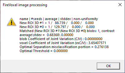
Used to estimate nonuniformity using two distinct tissues.
Requires two ROI layers, one in each tissue, with blobs uniformly
distributed over the image. Returns basic statistics for each ROI,
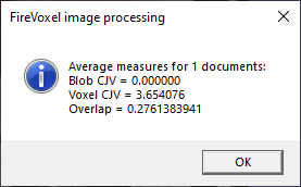
including number of seeds, average seed intensity, standard deviation,
and non-uniformity (Fig. 20.8).
Also provides measures derived from matched blobs:
contrast average\stdev. ADD DETAILS
Fig. 20.8 Results of Measure {CV, CJV, Spillover}.
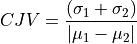
Blob Coefficient of Joint Variation (CJV): Defined from two set of
regions, delineated by expert observers in areas of known, uniform
tissue throughout the imaged organ (20.2).
where and are the average values,
and and
are standard deviations of intensity over the two regions. CJV
quantifies the intensity variability in each set and controls for the
potential undesirable loss of tissue contrast by the algorithm. CJV is
quantified before and after correction, a decrease in CJV reflects
decreased nonunformity.
Voxel CJV: vxCJV – similar quantity calculated… ADD DETAILS
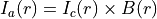
 is the acquired image,
  is the corrected image
and
is the corrected image
and  is the bias field. To find the corrected image, we need to estimate
the bias field.
is the bias field. To find the corrected image, we need to estimate
the bias field.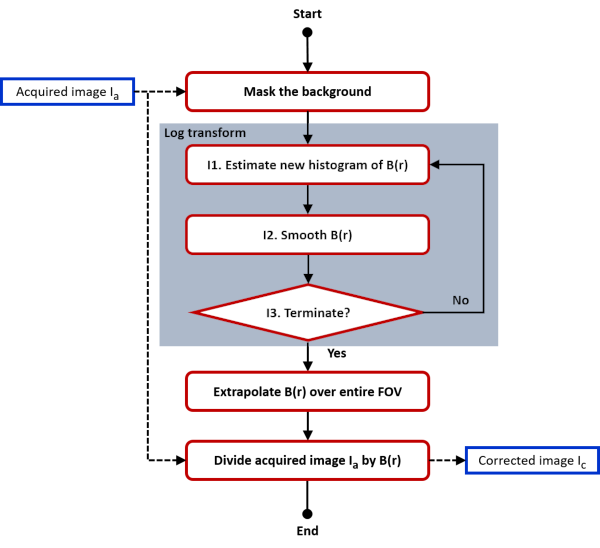
 .
.
 and
and  are the average values,
and
are the average values,
and  and
and  are standard deviations of intensity over the two regions. CJV
quantifies the intensity variability in each set and controls for the
potential undesirable loss of tissue contrast by the algorithm. CJV is
quantified before and after correction, a decrease in CJV reflects
decreased nonunformity.
are standard deviations of intensity over the two regions. CJV
quantifies the intensity variability in each set and controls for the
potential undesirable loss of tissue contrast by the algorithm. CJV is
quantified before and after correction, a decrease in CJV reflects
decreased nonunformity.