This section describes commands and options that control how the images
are displayed in FireVoxel. These commands include navigation through
slices and dynamic frames. These tools do not modify the image data,
but only change how the images are displayed. Customized views can be saved
as FireVoxel documents.
Many of these commands are available under the View tab on the main menu.
Selected commands are also accessible through the Toolbar.
Additional tools for adjusting the appearance of layers
(such as the layer order, visibility, ROI color, and color map options)
are available through Layer Control.
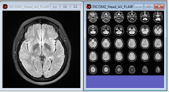
Fig. 9.1 The same volume in Slice View and Film View.
Images loaded in FireVoxel can be displayed in Slice View, when only one
slice is shown in the document window, or Film View, when all slices are
shown as tiles in the same document window (Fig. 9.1).
If the document is dynamic, Film View displays all slices at the same value
of dynamic variable (such as time, b-value, echo time, etc.).
To switch back and forth between the Slice and Film views, double-right-click
anywhere on the image.
To select the default initial view used when images are first loaded into FireVoxel,
use File > User Interface Options > Initial layout.
The user may navigate through the slices of a 3D volume by using the up and down
arrow keys on the keyboard or scrolling up or down the mouse wheel.
If the image is 4D, these actions enable viewing slices of a 3D volume
at a single dynamic frame.
To navigate through dynamic frames (such as time points or b-values), the user
can press the right and left arrow keys. In Slice View, the same slice will be
displayed at consecutive values of dynamic variables. In Film View, all slices
will also be displayed at each value of dynamic variable.
Creates a copy of the active document window in a new window. The
original window is renamed [name]:1 and the new window is named
[name]:2, etc. Each view can be manipulated independently and saved
separately.
Selects all vector entities (vector ROIs, polylines, and spline contours)
in the active document. With all vector entities selected, clicking anywhere
outside the vectors deselects all of them. Clicking any vector entity selects
that entity and deselects the others.
CAUTION: No file save dialogue. Any unsaved changes may be lost.
Closes the active document.
To avoid losing unsaved work, close each document by clicking the cross
in the upper right corner. Alternatively, close FireVoxel, in which
case the file-save dialog will be shown for each document one by one.
9.4.1. Set projection for this view (View & Toolbar)
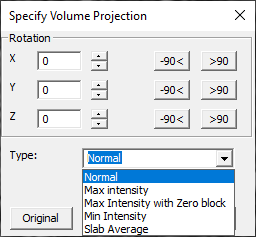
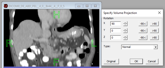
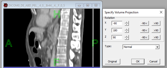
Opens a dialog panel (Specify Volume Projection, Fig. 9.3)
to configure orthogonal projection for the current document window.
Clicking View Projection icon opens the same panel.
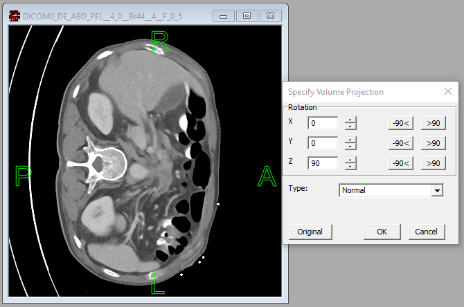
The top part (Rotation) contains boxes to enter angles (in
degrees) of rotation about X, Y, and Z axes. Orthogonal rotations can be
applied by clicking buttons +/-90 (degrees) (Fig. 9.4,
Fig. 9.5, Fig. 9.6).
Fig. 9.6 Projection at angles about X, Y, Z axes.
Clicking Original restores the original orientation.
The Type dropdown menu offers the choice of several types of views:
Normal (regular rotation, default), Max Intensity (maximum intensity projection),
Max Intensity with Zero block, Min Intensity (minimum intensity projection),
Slab Average (each voxel contains average signal at that location over the entire slab).
ADD DETAILS
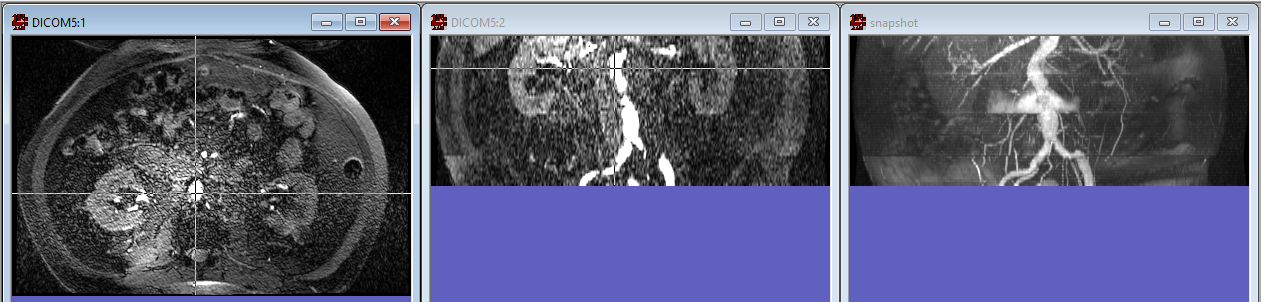
Opens a new document window (named snapshot) with the maximum
intensity projection (Fig. 9.7).
The snapshot has the same in-plane dimensions as
the original image, but contains only a single slice.
The snapshot cannot be converted back into the original image. In contrast,
maximum intensity image obtained using Set projection with Type
> Max intensity can be reset to the original image by selecting
Type > Normal.
Fig. 9.7 MR angiography axial and coronal views (left and center, respectively)
and coronal maximum intensity projection snapshot (right).
Clicking Display orthogonal projectionstoolbar icon opens document windows with orthogonal
projections complementary to the active document window.
For example, if the active document window displays an axial view,
the command opens two new document windows showing coronal and sagittal views.
By default, the new windows are tiled.
If the View Convention is Radiological (left side on the right),
Display orthogonal projections opens two additional windows
(for a total of three windows, including the original).
If the View Convention is Neurological (right side on the right),
Display orthogonal projections opens three additional windows:
the orthogonal projections plus the original projection in
left-side-on-the-left orientation (for a total of four windows,
including the original).
If the user clicks Display orthogonal projections icon two
or more times (with the same or different windows activated),
no new windows are opened besides the original set,
although document windows may be re-tiled after each icon click.
Zoom in on a rectangular selection with a mouse. To launch the tool,
select View > Zoom by window or click icon
(cursor becomes a magnifying glass). To use, click the image,
drag the mouse to expand a white dashed rectangle and release the mouse button.
Tool quits upon mouse release. To undo and return to the original view,
use View > Zoom All.
9.5.2. Zoom in/out with fixed upper left corner (View & Toolbar)
Zoom whole image relative to the upper left corner. To apply, select
View > Zoom in or Zoom out or click
icons or .
Repeat until a desired zoom level is reached.
Toggles on/off (checked/unchecked) visibility of vector ROIs and
polylines in the active document window (or current view if several
orthogonal projections are open).
Toggles on/off visibility of image layers and raster ROI layers in the
active document window (or current view if several orthogonal
projections are open).
Toggles on/off visibility of a rectangular grid.
Opens dialog (Specify Grid Step) with a box for entering
the Grid Step in millimeters.
Displays a square grid of green lines spaced by grid step in row and
column dimensions. The grid is shown for all slices, but only for the
current view (if orthogonal projections are displayed). To change the
grid step, use this command twice and enter a new grid step.
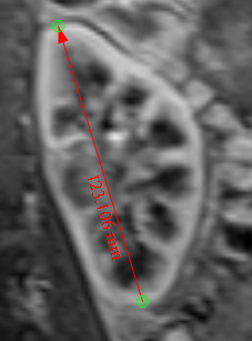
For a vector (a two-point polyline), toggles on/off the visibility
of the length of the segment between two points. The length
(in millimeters) is displayed next to the polyline as a red number
(Fig. 9.8).
For a sector (a three-point polyline), toggles on/off the angle
measure, displayed as a green number.
Opens a panel (Polyline and Spline properties) for adjusting
parameters of vector polylines and splines. This panel can also be open
by double-clicking a polyline or spline. This panel is described in detail
in Trace section on Magnetic Trace tool.
Clicking Play 4D experiment icon to display
the dynamic frames of the current slice consecutively
for a user-specified time interval.
Opens dialog (Specify Interframe time delay (.001 sec precision))
with a box for entering the time during which each frame is shown.
Clicking OK starts the sequence of views. The cursor turns into a blue wheel.
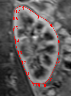
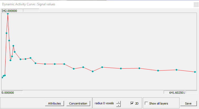
Clicking Display voxel TAC icon
opens a panel to view the time-activity curve (TAC) at the current voxel
(Dynamic Activity Curve: Signal values, Fig. 9.10).