This section describes FireVoxel’s tools for the analysis
of diffusion-weighted MRI (DWI).
A typical DWI experiment involves:
4D images acquired using diffusion-weighted (DW) sequences, usually spin
echo echo-planar imaging sequences (SE-EPI), at two or more diffusion
weighting factors (b-values, in s/mm2) as the dynamic
dimension, and
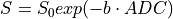
Model fitting of DWI data to calculate the apparent diffusion
coefficient (ADC, mm2/s) and other parameters of tissues
of interest.
FireVoxel offers a set of tools for the analysis of DWI data,
including image loading, preview, signal visualization, motion
correction, and model analysis.
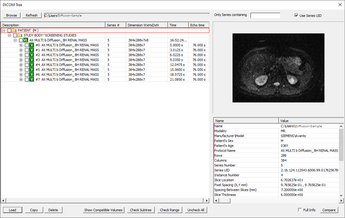
DW images in DICOM format can be loaded into FireVoxel as 4D datasets
using File > Open DICOM Single Document or
Open DICOM Multiple Documents (DICOM Tree dialog, Fig. 30.1).
Fig. 30.1 DICOM Tree dialog for loading DWI dataset.
In the DICOM Tree dialog, DW images are organized by PATIENT, STUDY,
4D volume lists (VL, ), and 3D volumes (V, ).
The user may load the entire 4D series (VL) or individual 3D volumes (V)
by checking the boxes next to the corresponding titles and clicking Load.
If no boxes are checked, the entry highlighted with a red box will be loaded.
For most MRI systems, the b-values should be automatically read from
the DICOM header (Diffusion b-value Attribute (0018,9087)).
Please contact the FireVoxel team about any issues
with image loading.
It is important to verify the correctness of the b-values
once the images are loaded into FireVoxel. To do this, scroll through the images
using the Right and Left arrow keys on the keyboard and check the b values
displayed in the status bar in the lower left corner of the main software window
(Fig. 30.2). To scroll through slices, use Up and Down arrow keys.
Fig. 30.2 The status bar in the lower left displays the current b-value.
The signal change with b-value can also be viewed using Play 4D experiment
tool on the main toolbar. The local signal behavior
can also be visualized using Voxel Time Activity Browser .
Before proceeding with the analysis, the user is advised to check the images
for any issues, for example, motion artifacts, and decide whether any preprocessing,
such as motion correction, may be necessary.
If the images are affected by motion, the user may use 4D coregistration
tools to align images.
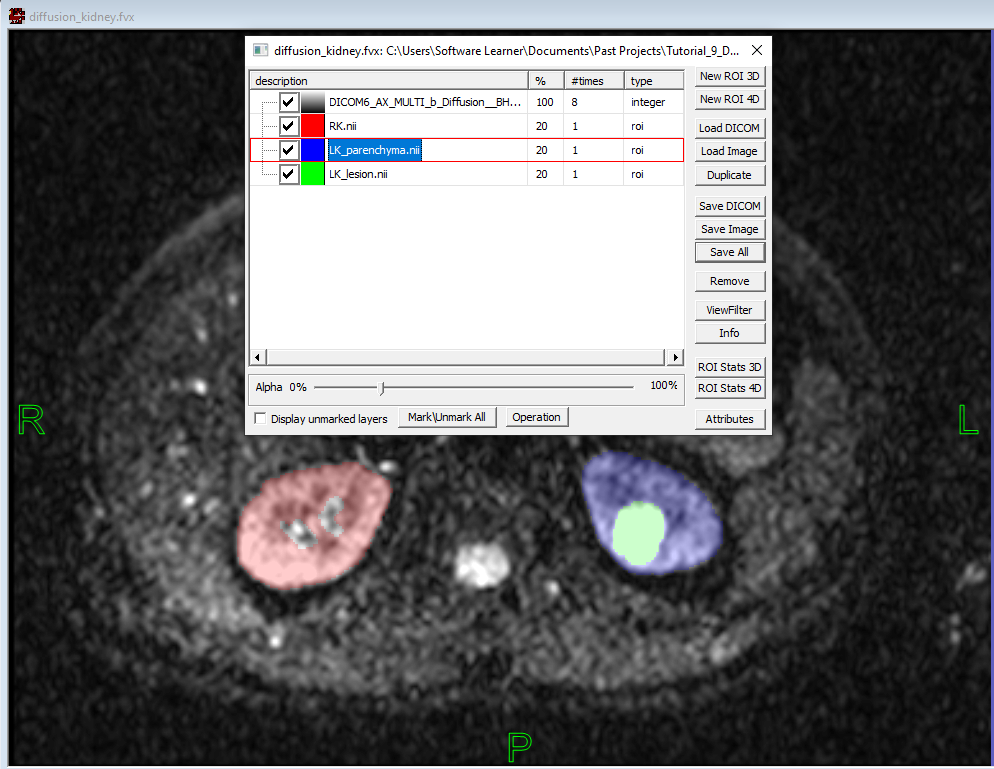
Prior to modeling, it is recommended to segment the organs or tissues
of interest using FireVoxel’s segmentation tools and perform initial
voxel-based analysis within these ROIs (Fig. 30.3).
Fig. 30.3 The ROIs allow the user to examine parameters of tissues of interest.
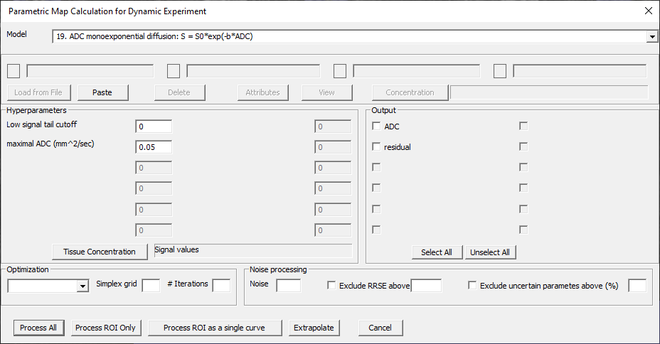
The analysis of DWI data may be performed using Dynamic Analysis >
Calculate Parametric Map command, also available via
toolbar icon. The command opens a dialog panel for setting up the model
analysis (Parametric Map Calculation for Dynamic Experiment,
Fig. 30.4).
Fig. 30.4 Calculate Parametric Map dialog for DWI.
The top part of the panel (labeled Model) contains a drop-down menu
with a numbered list of models compatible with the current dataset.
The compatibility between data and models is determined by FireVoxel
automatically based on the DICOM header information. Models that are not
compatible with the current dataset are not shown.
The following models are compatible with the DWI data:
This series of text boxes allows the user to specify the fixed input
parameters (referred to below as hyperparameters) and the bounds
of the fitted model parameters:
Low signal tail cutoff – If signal intensity falls below this
cutoff value, the data at the corresponding b-value and all higher b-values
are discarded from fitting.
Maximal ADC (mm^2/sec) – Upper limit on the ADC value.
[Tissue Concentration – Not relevant to DWI processing.
Opens Concentration Conversion dialog for setting up the conversion
from signal intensity to contrast concentration in contrast-enhanced CT
and dynamic contrast-enhanced MRI experiments.
By default, unconverted Signal values are selected, so no further action
is needed for DWI analysis. This option will be removed in future builds.]
These checkboxes allow the user to select the parameters that will be
returned as the results of model analysis. At least one output parameter
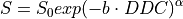
must be selected. For curve fitting models, the output parameters also include
a measure of goodness of fit, such as the root-mean-square error
This block controls the optimization options for the curve fitting models
(for both voxel-based and average curve fitting analyses, see Fitting Options).
[Optimization method] – Dropdown menu with a choice of: 1) Simplex optimization
or 2) Global optimization.
Simplex optimization is based on the simplex Nelder-Mead (or amoeba) method.
As a heuristic, it finds an optimal solution by iteratively replacing the worst
solution with a better solution at each step. The simplex method starts from
multiple grid points for fitted parameters, which ensures a more optimal solution,
but is not guaranteed to yield the global optimum. The precision of the simplex
solution is determined by a combination of the number of simplex grid points
and the number of iterations (see Simplex grid and #Iterations below).
Simplex optimization can work efficiently with multiparameter models.
In FireVoxel, all convolutional models currently use simplex optimization.
Global optimization is based on interval arithmetic, branch-and-bound approach
that always searches for a guaranteed global optimum. The precision of global
optimization is controlled by fitted parameter bounds (see Hyperparameters)
and the maximum allowed number of iterations. Global optimization provides
the exact solution bounds on the globally optimal parameters and fitting residual
(which heuristic methods, such as simplex optimization, cannot provide).
With increasing number of iterations, the solution bounds become tighter.
For models with multiple parameters, global optimization may become impractical
because of the high computational cost.
Simplex grid – Number of grid points Ng (typically 3 to 5)
for simplex optimization. For the monoexponential model, the grid points
are constructed by dividing the full ADC range from 0 to the maximum ADC
into (Ng-1) equal subintervals. For other models, Ng
applies to each of the fitted parameters.
#Iterations – Maximum number of iterations used as a stopping criterion
in simplex fitting. Higher numbers may help achieve a better fit but
will also require longer processing times.
Sets the parameters of noise and excluding unreliable data and/or results:
Noise – Noise level.
Exclude RRSE above – Checkbox and text box (for cutoff value) –
Exclude voxels with poor quality fit. If the box is checked,
replace with VOID any voxel for which RMSE is above the cutoff entered
in the text box. Trial and error is often used to establish the desired cutoff.
Exclude parameters above (%) – Checkbox and text box (to enter percent cutoff) –
Exclude voxels that yield exceedingly large or negative parameters.
If the box is checked, replace with VOID any voxel where ADC is greater
than percent cutoff as defined by maximum ADC.
30.5.6. Fitting options: Process All, Process ROI Only, Process ROI as a single curve
These buttons at the bottom of the panel enable the user to select
how the model analysis is performed: on a voxel-by-voxel basis over
the entire image, or within an ROI, or for an ROI-averaged curve.
The available options depend on the presence of a visible ROI layer
(or layers). If ROIs are invisible or not present at all, only the
entire image can be modeled (voxel-by-voxel or as an average curve).
If multiple ROI layers are visible and one of them is active, the model
analysis is performed for the active ROI. If ROIs are visible, but none
of them is active, modeling is available either for the entire image or
for all of the ROI-averaged curves.
Process All – Fit the entire image voxel by voxel. For each output parameter,
the result will be displayed as a color map residing in a new, automatically
created real-valued layer. These new layers will be placed on top of all other
layers in the same document window as the original data.
Process ROI Only – Enabled when the active layer is a visible ROI.
The model analysis is performed on a voxel-by-voxel basis within the ROI.
If more than one ROI is present, but none of them is active, this option
is not available. The results will be returned as new, color map layers,
as in Process All.
Process ROI/volume/All ROIs as a single curve – The functionality depends
on the active layer:
1) The active layer is a visible ROI – Fit the curve obtained by averaging
the signal within the active ROI.
2) The active layer is an image layer and no ROIs are visible or present
– Fit the signal averaged over the entire volume.
3) The active layer is an image layer, and multiple visible ROI layers
are present – Fit the curves obtained by averaging each visible ROI.
Extrapolate – Create an extrapolated 4D volume corresponding to
the user-specified values of the dynamic variable (b value for DWI),
with signal in each voxel computed based on the model formula and fitted
parameters. The extrapolated 3D volumes are added to the original image
set and displayed in a new document window titled
[original document]_extrapolated.
The results correspond to the fitting options selected in the previous step:
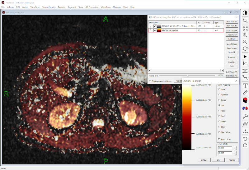
Process All – Parametric maps, displayed as color maps,
for the entire image. The appearance of the color maps can be customized
using ViewFilter command on the Layer Control panel (Fig. 30.5).
Fig. 30.5 Process All results showing whole-image ADC map.
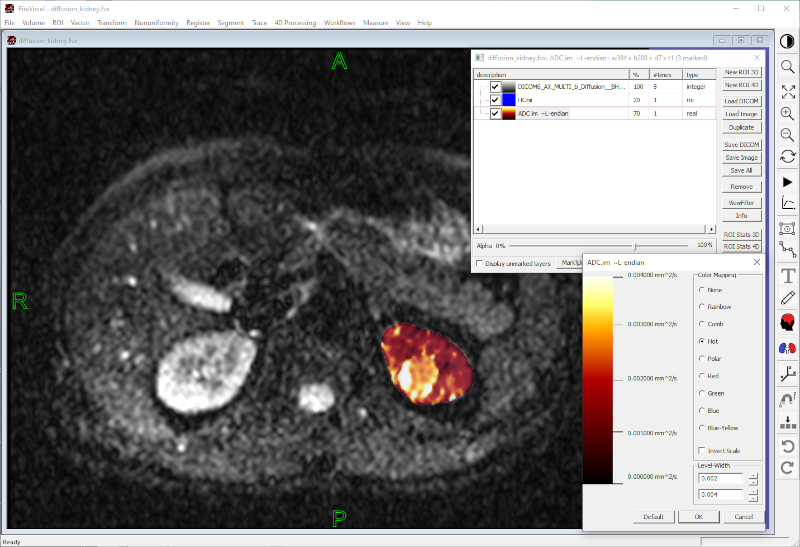
Process ROI Only – Parametric maps within the filled (non-zero)
ROI voxels; all other voxels remain fully transparent.
Again, the appearance of the color maps can be customized using
ViewFilter (Fig. 30.6).
Fig. 30.6 Fit ROI Only results showing map of ADC for the right kidney.
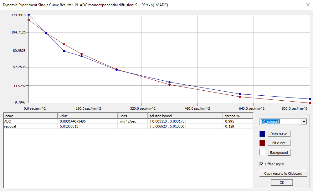
Process volume/ROI/ROIs as a curve – Opens the output panel
(Dynamic Experiment Single Curve Results: [Model name],
Fig. 30.7). The panel consists of three parts.
Fig. 30.7 Dynamic Experiment Single Curve Results panel.
The top part of the panel displays a plot of the signal data
and the model fit as a function of the dynamic variable (for DWI b-value,
s/mm2). The bottom right part shows the current ROI (and a dropdown
menu to select other ROIs, if multiple ROIs were fitted). Below the ROI menu are
the color swatches for the data curve, fit curve, and the plot background.
The buttons next to the color swatches open the standard color picker
for selecting the colors of the curves and the background.
The bottom left part under the plot contains a table of fitted parameters
with the columns showing parameter name, fitted value, and units
(if applicable). For Model 19, the table lists the ADC and residual
as the output parameters.
For global optimization, the table also shows the lower and upper solution
bounds [LB, UB] on the globally optimal parameter value OV and
percent spread = 100%*max(OV-LB, UB-OV)/OV.
Offset signal (checkbox) – Toggles on/off the vertical axis offset.
If checked, the vertical axis range is restricted to the interval
between the smallest and largest value of the data or fitting curve.
If unchecked, the vertical axis range is from zero to the largest data/fit value.
Copy results to clipboard – Copies fitted parameters to the clipboard
and makes them available for posting into a text file or spreadsheet.
For each ROI, each parameter is recorded in a separate line (ROI name,
parameter name, fitted parameter value, and units, if applicable).
OK – Closes the panel.
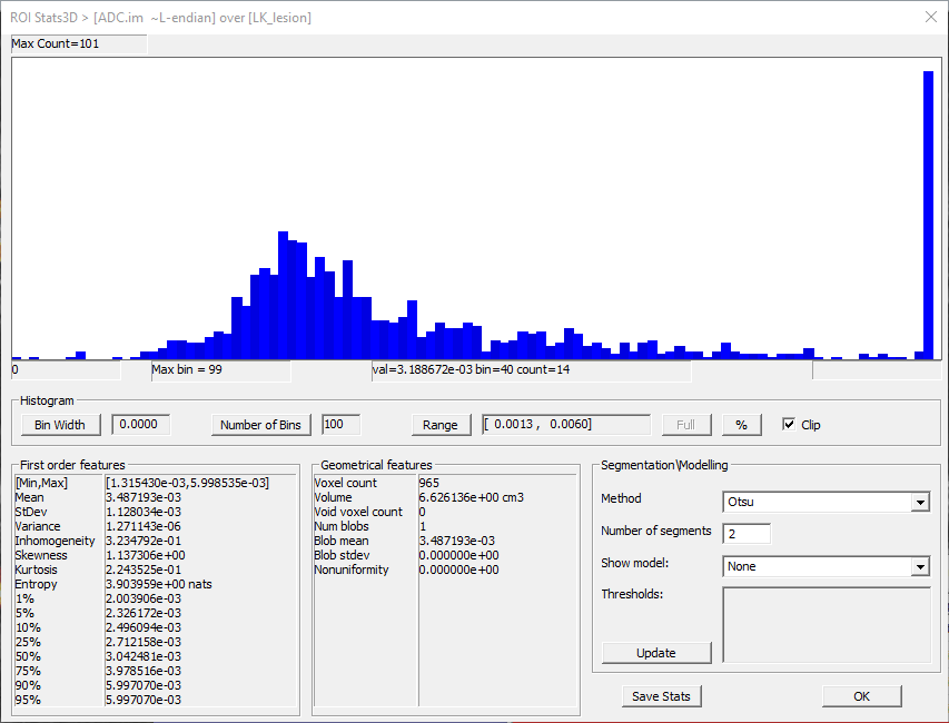
30.5.8. Analyzing parametric maps with ROI Stats 3D
To explore the ADC voxel values within an ROI, make sure that this ROI
is the only visible ROI layer and the ADC map is the active layer,
then click ROI Stats 3D on the Layer Control panel. This command opens
a panel (ROI Stats 3D) that provides the histogram, selected features,
and other statistics of the parameter distribution.
Fig. 30.8 The ROI Stats 3D panel showing ADC statistics within the left kidney ROI.
The top part of the panel shows the histogram of the voxel distribution
of the parameter values. The options controlling the histogram are
located below the histogram. These options include the Range,
Number of bins, and Bin Width.
By default, the full range of values is displayed. To adjust the range,
click Range to open dialog showing the lower and upper bounds and type
new values. If Clip box is checked, the values outside the Range
are not included into the histogram and from statistics calculation.
This is reflected in the first order features and ROI voxel count
(under Geometrical features). In response to the change of Range,
the Number of bins is automatically updated (if Bin Width stays
unchanged).
The range may also be set via specifying the low and high percentile
bounds to be displayed (by clicking the % button and entering
the corresponding values). Clicking Full restores the full range
of values included into the histogram.
The lower left part of the panel lists the first order features
of the voxel values distribution, including the mean, standard deviations,
etc., as well as a selection of percentile values between 1% and 95%.
All values are displayed in scientific notation, e.g., mean
ADC = 3.487193e-03 = 0.003487193.
Geometrical features list the voxel count and ROI volume and other parameters.
The Segmentation\Modeling options on the lower right enable partitioning
(segmentation) of ROI voxels into subgroups, such as viable tissue versus
necrotic tissue, based on the voxel value distribution. Voxels within
each subgroup are presumed to have similar parameter values.
Clicking Save Stats opens a text file with the main statistical results
(named RoiStats3D.txt), including ROI volume, first order features,
and histogram. By default, this file is created in FireVoxel’s Temp
directory, but can be saved in any user-selected directory.
 ), and 3D volumes (V,
  ).
The user may load the entire 4D series (VL) or individual 3D volumes (V)
by checking the boxes next to the corresponding titles and clicking Load.
If no boxes are checked, the entry highlighted with a red box will be loaded.
).
The user may load the entire 4D series (VL) or individual 3D volumes (V)
by checking the boxes next to the corresponding titles and clicking Load.
If no boxes are checked, the entry highlighted with a red box will be loaded.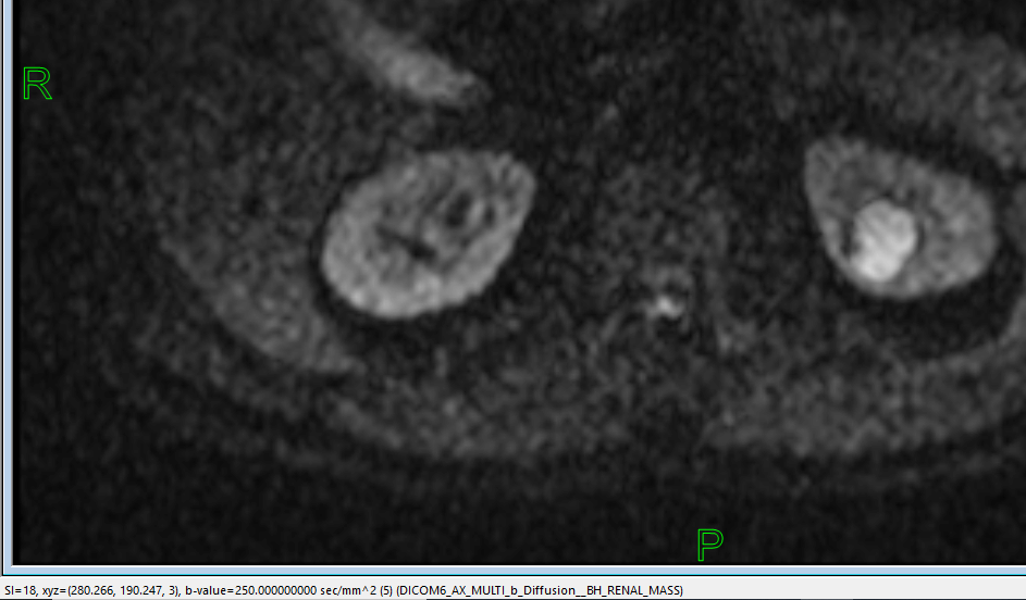


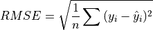
 and
and  are the signal data and model fit values,
respectively, at
are the signal data and model fit values,
respectively, at  -th value of the dynamic variable
(
-th value of the dynamic variable
( ).
).