In dynamic imaging that involves administration of tracers or contrast
agents, such as dynamic PET, dynamic contrast-enhanced (DCE) MRI and DCE
CT, serial images are acquired and analyzed to derive functional
information about organs and tissues. The analysis is often performed
using compartmental models, which require knowledge of the input
functions driving the system. The input function (IF) is usually
determined as the time-activity curve (TAC), or contrast concentration
curve, in a blood vessel feeding the organ or tissue. The input function
can be measured in a manually-drawn ROI or derived analytically by
selecting voxels based on the characteristics of their time-activity
curves.
FireVoxel offers a semi-automatic tool to determine the IDIF with
minimal user interaction. The user must first draw a vector ROI (seed) to
initialize the process and then use Dynamic Analysis > Image Derived
Input Function to customize and run the IDIF tool. The resulting IDIF
(signal versus time data) can be saved as a text file or pasted into
other applications.
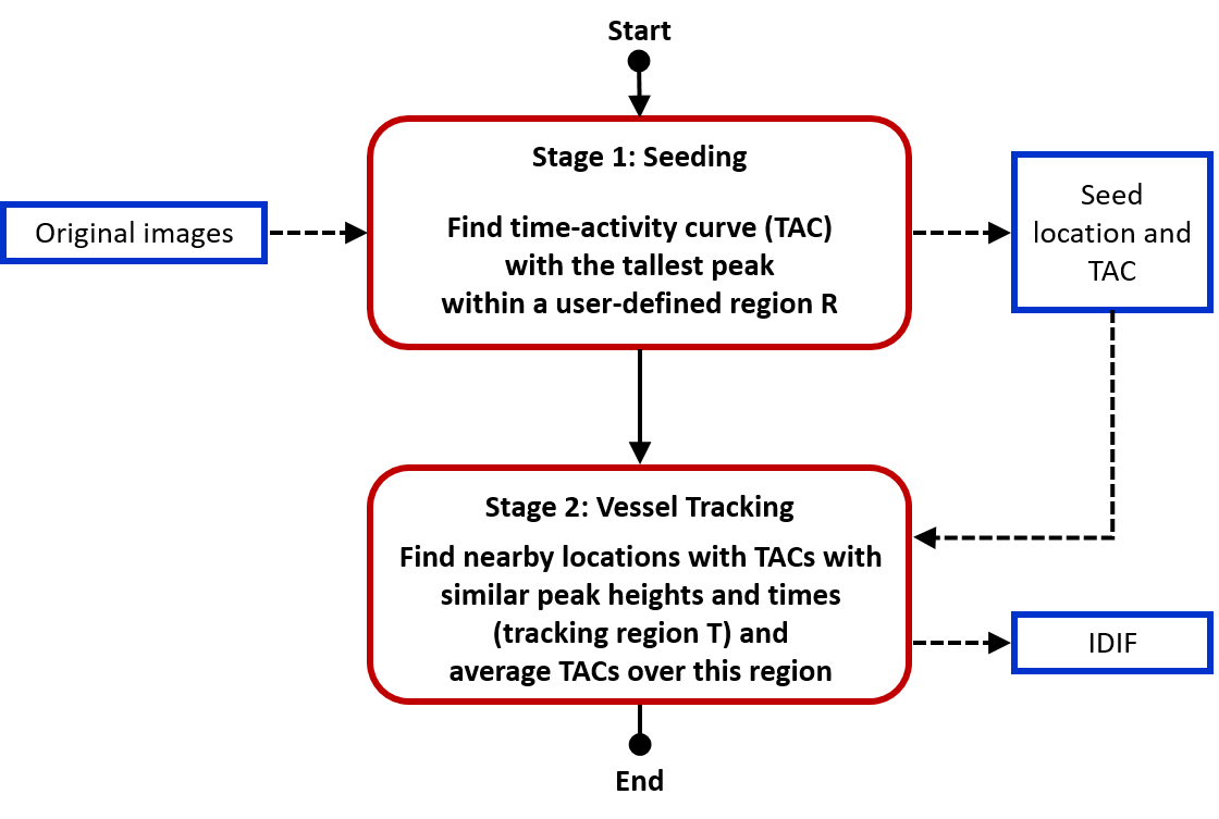
The IDIF algorithm has two stages: 1) seeding and 2) vessel tracking
(Fig. 36.1).
In the seeding stage, the algorithm finds a location where
the time-activity curve (signal versus time curve) has the tallest peak
within the user-defined seed region.
In the vessel tracking stage, this starting location and its reference curve
are used to initialize the search for nearby voxels with similar time-activity
curves. The candidate curves are compared with the reference curve.
The locations where candidate curves are similar to the reference curve are added
to the vessel tracking region. The average time-activity curve of the tracking region
serves as the IDIF.
The user first loads the dynamic images into FireVoxel
using, for example, File > Open DICOM.
In most cases, FireVoxel will read the time points automatically
from the DICOM image header.
The user then defines a vector ROI enclosing the blood vessel using
Vector > Construct Vector ROI
or the toolbar icon.
The position of the VROI can be adjusted in three dimensions using
Display orthogonal projections.
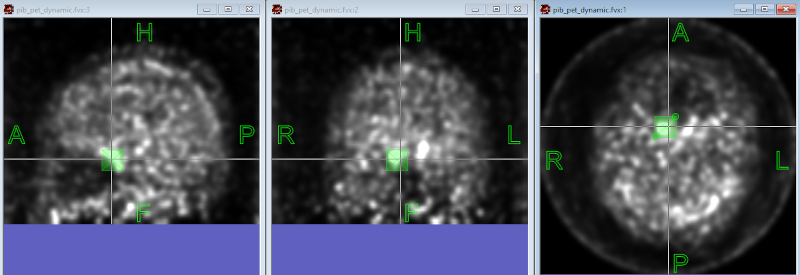
The ROI does not need to conform to the vessel, but only delineate
the area in which the vessel is located (Fig. 36.2).
Fig. 36.2 Vector ROI (green square) on PET image (in 3 projections) to initialize the IDIF tool.
The user must keep in mind various confounding factors that may complicate
the identification of the IDIF voxels. For example, the presence of the veins
within the seed ROI may distort the resulting arterial input function.
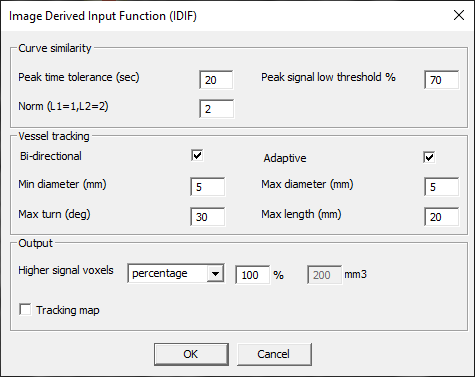
The top part, labeled Curve similarity, contains parameters that
control the comparison between the candidate curves with the reference
curve:
Peak time tolerance – Maximum time difference between the peaks
of the candidate curve and the reference curve. A candidate curve
with a peak within this interval is considered further.
Peak signal low threshold – Minimum peak height (as percent of the
reference curve peak height) that the candidate curve must have to be
considered further. If the threshold is 80%, then candidate curves
must have peaks of at least 80% of the reference curve peak height.
Norm (L1=1, L2=2) – The user can select L1 or L2 norm
to evaluate the difference between the candidate curve
and the reference curve.
The middle part, Vessel tracking, sets the parameters of the vessel
tracking process (Fig. 36.4).
Bi-directional [tracking] – Checkbox that toggles between the entire
tracking region or only its part being used to derive the input function.
The algorithm always tracks the vessel in both directions away from the
seed location. If Bi-directional option is checked, both arms of the
tracking region are included. If Bi-directional option is unchecked,
only the longer arm of the tracking region is retained.
Adaptive – Checkbox that toggles between adaptive and regular modes.
In Adaptive, the reference curve is equal to the average curve over
the tracking region and is updated on every tracking step. In Regular
mode, the reference curve is equal to the seed curve and is constant
throughout the tracking process.
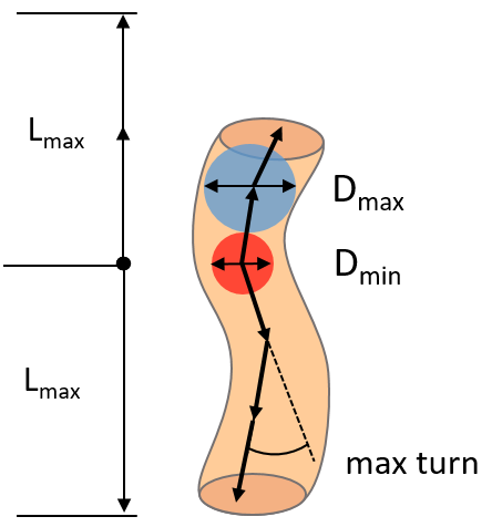
Minimum and Maximum diameters (mm) – Set the limits for the
diameters (Dmin, Dmax) of the candidate spheres
at every tracking step to account for possible variation of the vessel
width over the tracking region.
Maximum length (mm) – Sets the maximum length Lmax
of each arm of the tracking region.
Maximum turn (deg) – Angle (in degrees) that limits the angle by
which the direction of the tracking region can change from one tracking
step to the next. This ensures that the tracking region follows a smooth
course along the vessel.
The lower part of the panel, labeled Output, contains the parameters
controlling the results.
Higher signal voxels – Dropdown menu to select a percentage of
voxels, or a volume in cubic millimeters, that will be used to derive
the input function.
Tracking map – Checkbox to create a new layer with an integer-valued
color map of the tracking region showing its growth at each step.
This map will be created in addition to the tracking region mask and may be
helpful in understanding the tracking process and adjusting its parameters.
The IDIF tool outputs include 1) IDIF ROI and 2) tracking map
(if Tracking map box was checked in IDIF dialog).
The IDIF ROI and tracking map cover the same voxel locations, but the ROI
is a binary mask and the tracking map is an integer-valued image shown as
colormap.
The IDIF ROI is returned in an automatically created layer labeled IDIF.
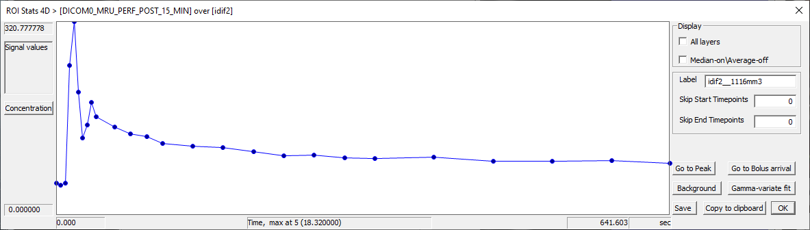
The average signal over the IDIF ROI will be displayed
in the ROI Stats 4D panel
opened automatically (Fig. 36.5).
This curve can be saved as a text file or copied to clipboard using
Save and Copy to clipboard commands, respectively,
in the lower right corner of the panel.
Fig. 36.5 IDIF is automatically displayed in ROI Stats 4D panel.
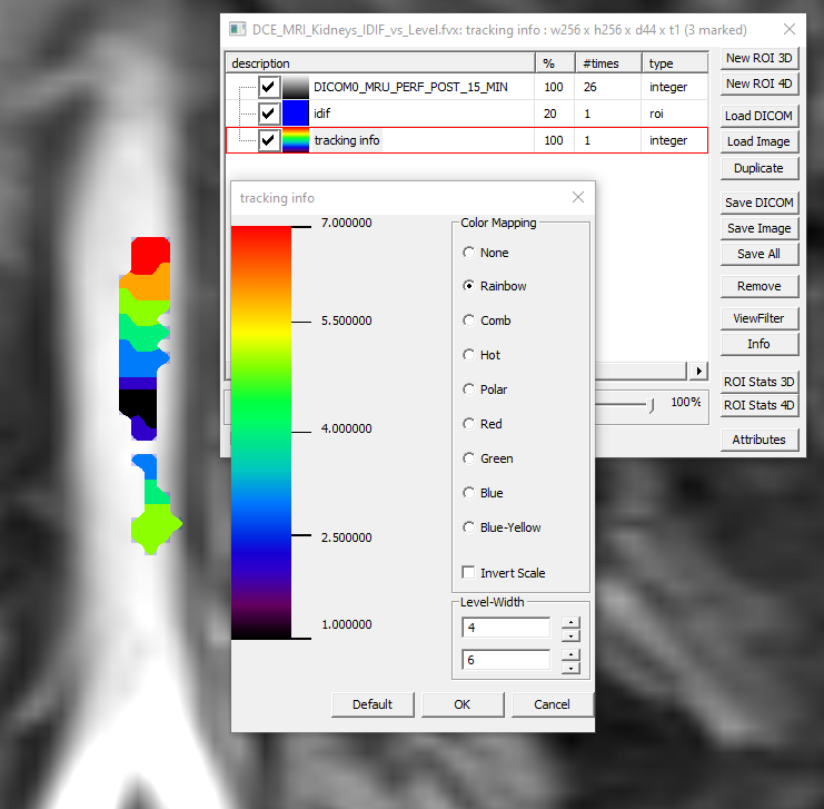
The tracking map is placed in a layer labeled tracking info.
By default, the tracking map is displayed in the Rainbow color map, with
the seed sphere shown in black and other colors indicating areas added at each
tracking step (Fig. 36.6).
The IDIF ROI and tracking map layers are best saved within the FireVoxel
document, but can also be saved separately
(see File > Save Active Layer as Image or
Layer Control > Save Image).
Prior to using the IDIF tool, the user defines a rectangular seed
(vector ROI) enclosing the vessel. The user then selects Dynamic Analysis >
Image Derived Input Function to launch the IDIF tool.
The IDIF algorithm works in two stages: 1) seeding and 2) vessel tracking.
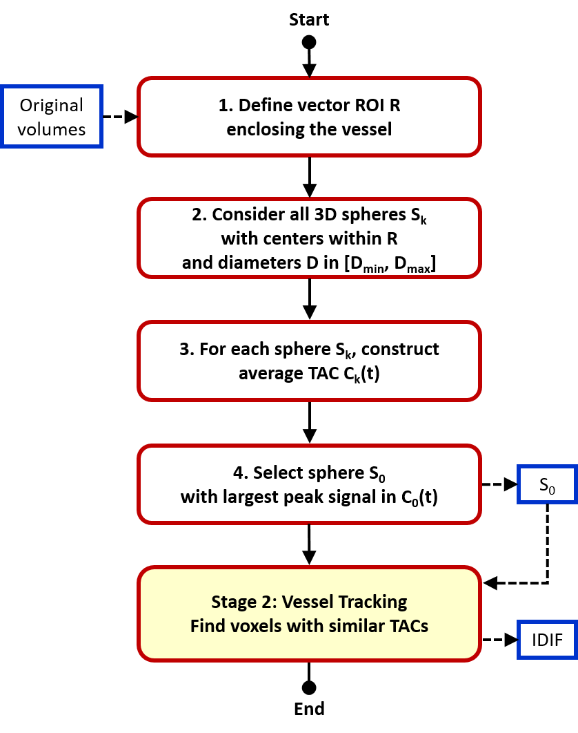
1. Seeding (Fig. 36.7).
The algorithm considers all 3D spheres with centers inside the seed region
and with diameters within a user-specified interval.
For each sphere, the average time-activity curve is constructed by averaging
all voxel curves within the sphere. The sphere with the tallest peak is selected,
and its location and time-activity curve are used as the seed to initialize
the next step.
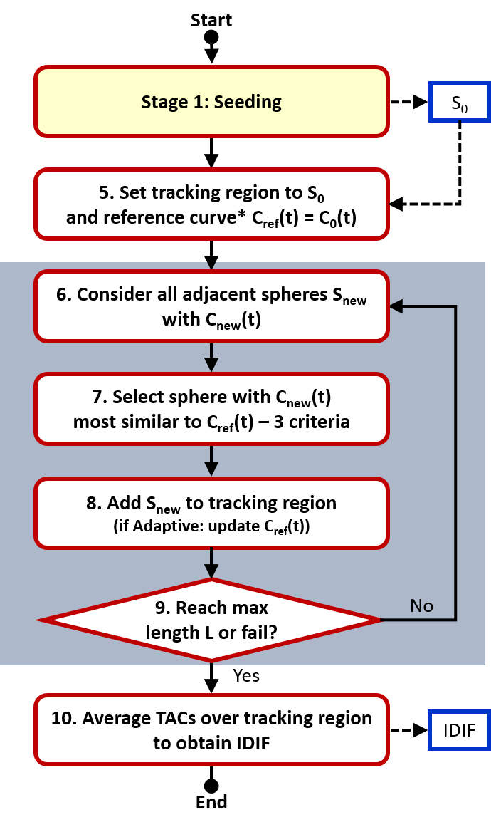
2. Vessel tracking (Fig. 36.8).
First, a three-dimensional tracking region is initialized with the seed sphere
as the starting location. The reference time-activity curve is set equal
to the seed curve.
The algorithm has two modes, regular and adaptive.
In regular mode, the reference curve remains equal to the seed curve
throughout vessel tracking. In adaptive mode, the reference curve is set equal
to the average curve over the tracking region and is updated on every iteration.
Next, vessel tracking begins iterations. At each step, the algorithm
considers all spheres adjacent to the current tracking region and
selects the sphere with the time-activity curve most similar to the
reference curve based on the following three criteria:
The peak height of the candidate curve must exceed the user-specified
threshold percentage of the reference curve peak.
The peak time of the candidate curve must be within the time tolerance
interval of the reference curve peak time.
If the first two conditions are met, the candidate curve must yield the
smallest difference between itself and the reference curve (expressed
as the L-norm).
The sphere that satisfies these three conditions is then added to the
tracking region. In adaptive mode, the reference curve is updated to the
average curve of the newly expanded tracking region.
This sequence is repeated until the user-defined vessel length is
reached or tracking fails. After vessel tracking is finished, the
image-derived input function is determined as the average time-activity
curve over the filled voxels in the tracking region.