The Volume tab contains commands for manipulating 3D and 4D datasets.
This includes cropping, signal scaling, smoothing, application of
edge-enhancing filters and so on. Also included in this tab are tools for
conversion of numeric data type between integer and real and changing data
dimensions.
These commands automatically adjust the grayscale window center
and width to the optimal settings for selected conditions.
See also View > Grayscale Window
for details of grayscale window center and width settings.
This operation is defined for integer and real volumes only.
The optimal window center/width setting is defined as follows.
First, all non-void (non-transparent) voxels are sorted into a list
by their signal intensity values. Next, a fixed percentage of all voxels (0.5%)
is removed from the top and the bottom of the list. For the remaining voxels,
the range between the lowest and highest signal values is taken to be
the optimal window width and the midpoint of this range as
the optimal window center.
Automatically adjusts window center and width to the values optimal
for viewing of the current timepoint (time frame). May be convenient
for viewing dynamic series in which image intensity varies in a wide range,
such as dynamic contrast-enhanced MRI or CT images showing high signal enhancement
in blood vessels during the passage of the contrast bolus with.
Automatically adjusts window center and width to the values optimal
for viewing of the active, visible ROI layer.
If the document contains two or more ROI layers, but the active layer
is not an ROI, shows an error message (Ambiguous Layer Configuration).
Selects and displays the dynamic frame with the maximum information
within a raster ROI. Requires a 4D (dynamic) dataset and a single raster ROI.
If the document contains two or more ROI layers, shows an error message
(Ambiguous layer configuration). If the document contains no visible ROI,
displays the dynamic frame with the maximum information for the entire image.
In FireVoxel, by default, images (volumes) are compressed to save RAM.
Each slice of the volume is compressed separately using three-voxel
predictive coding combined with the
Huffman entropy encoder.
The compressed size of the entire volume is thus the sum of the sizes
of individual slices.
The size of the compressed volume is an indicator of how much information is contained
in the volume. The less uniform the signal within the volume, the more information
it contains and the larger the volume’s compressed size. A uniform volume (a volume
containing the same signal values throughout) has nearly zero compressed size.
This command advances to the timepoint where a 3D volume has the largest
compressed size. In dynamic contrast-enhanced studies, which consist of a series
of 3D volumes, the maximum information usually corresponds to the timepoint of
the maximum contrast enhancement.
Users may select non-compressed internal representation of the volumes via
File > User Interface Options > RAM Compress Integer volumes (uncheck).
Without compression, all slices and timepoints have the same amount of information,
and operations based on maximum information are not meaningful.
Selects and displays the time frame showing maximum image intensity
within the active vector ROI (VROI). If the VROI is not present, or multiple
VROIs are present, but none is selected, FireVoxel will show a corresponding
error message (if no VROIs: At least one seed is expected;
if multiple VROIs, none selected: With several seeds present,
a single one should be selected). The seed VROI may be 2D, 3D, or 4D.
Selects a user-specified subset of the original dataset.
Creates a new document window (named [original]_cropped) displaying
the selected subset.
15.3.1. Crop with 4D Vector ROI – Active Layer only
Requires a document with an active layer and an active vector ROI (VROI).
Selects a part of the active layer enclosed by the VROI.
Creates a new document window (named [original]_cropped) displaying
the selected subset of the active layer. The VROI is not copied
to the cropped document.
The active layer may contain an image (3D or 4D), raster ROI (3D or 4D),
or a color map. Even if the active layer is invisible, it will be cropped
and displayed as visible in the new (cropped) document window.
The VROI may be 2D, 3D, or 4D. A 2D or 3D VROI will crop a single slice, volume,
or dynamic frame on which it is defined. Similarly, a 4D VROI will crop only those
dynamic frames on which it is defined.
To adjust the dynamic frames, double left-click the VROI to open
VROI Properties panel and enter the dynamic index interval.
See Vector for details.
If multiple VROIs are present in the document, but none is selected,
the command shows an error message (More than one Vector ROI is present
and none selected).
If the document contains multiple layers, they are not included into
the cropped document. To crop multiple layers, use Crop with 4D Vector ROI —
All Layers.
Requires a document with one or more layers and an active vector ROI (VROI).
Selects a part of all layers in the document enclosed by the VROI.
Creates a new document window (named [original]_cropped) displaying
the selected subset of the original document. The VROI is not copied
to the cropped document.
The original document may contain images (3D or 4D), raster ROIs (3D or 4D),
or color maps. Both visible and invisible layers will be cropped, but
invisible layers will remain invisible in the new (cropped) document window.
The VROI may be 2D, 3D, or 4D.
A 2D or 3D VROI will crop a single slice, volume, or dynamic frame
on which it is defined. Similarly, a 4D VROI will crop only those dynamic
frames on which it is defined.
To adjust the dynamic frames, double left-click the VROI to open
VROI Properties panel and enter the dynamic index interval.
See Vector for details.
If multiple VROIs are present in the document, but none is selected,
the command shows an error message (More than one Vector ROI is present
and none selected).
Requires a dynamic (4D) image.
Selects a single frame (3D volume) at the current value of dynamic variable
(such as time, b-value, flip angle, inversion time, Dixon contrast, etc.)
Creates a new document window (named [original_image]_cropped) showing
the selected (cropped) volume.
The dynamic variable and dynamic index are shown in the status bar
at the bottom left corner of the software window (Fig. 30.2).
If the original document contains other visible layers (including ROI layers),
they are copied into the cropped document. The layers that are invisible
in the original document are not included into the cropped document.
Vector ROIs are not retained.
Requires a 3D or 4D image in the active document window.
Selects the current slice (e.g., slice number P) from the original document.
Creates a new document window (labeled [original]_slP) showing the selected slice.
If the original document contains a 3D image, the cropped image is a 2D slice.
If the original document contains a 4D image, the cropped image
is a 2D slice at all dynamic points of the original document.
All raster ROI layers (both visible and invisible) and vector ROIs are replicated
in the cropped document.
Requires a 4D image. Opens a dialog prompting the user to enter the indices
of the dynamic variable to be selected. These indices may be separated by commas
(e.g., 1, 3, 9) to select individual dynamic frames, or by dashes (e.g., 1-10)
to select a range of indices.
Creates a new document window (labeled [original]_cropped) with a 4D image
that includes the 3D volumes with the specified dynamic variable indices.
For example, the user selects time points 1, 3, 9 from a time series,
the cropped image will contain volumes at time points number 1, 3, and 9.
If the user selects dynamic points 1-10, the cropped image will contain
the first ten images of the dynamic series.
Requires a 4D image. Opens dialog prompting the user to enter an index (or indices)
of the dynamic variable of the 3D volumes that will be removed from the original 4D image.
Creates a new document window (labeled [original]_cropped) with a 4D image
in which the specified dynamic frames are absent.
If the dynamic variable is time (with the time points from t1=0 s
to tN), and the first K points are removed [t1, tK],
the time points of the remaining images [tK+1, tN]
are adjusted by subtracting tK+1 so that the time points
of the cropped image are in the interval of
[0 s, tN — tK+1].
If the original document contains invisible layers, they are not replicated
in the cropped document. However, visible layers (images, ROIs, maps) are retained.
Requires a document with an active layer (visible or invisible).
Opens dialog (Specify Pad size (mm)) to enter padding size in millimeters.
Creates a new document window (named [active_window]_pad) with padded image,
in which zero intensity voxels added to each dimension of the original volume.
The dimensions of the padded image are (w+p, h+p, d+p), where w, h, and d are
the width, height and depth of the original image (in mm), and p is the pad size.
If the image is 4D, each frame of the original dynamic series is padded.
The voxel size of the padded image is the same as the original voxel size.
The matrix of the padded image is increased by the number of added padding voxels.
Returns the noise values estimated using different methods for the image
in the active layer. Displays the results in FireVoxel image processing dialog.
Use Ctrl+C, Ctrl+V to copy and paste these results elsewhere.
Requires an integer image. Returns the value of effective noise.
This is effectively a 2D algorithm.
The algorithm scans all slices within the volume and for each slice
measures the average signal within a 2D window (10 mm x 10 mm).
The window with the lowest average signal and assumed to contain air.
The effective noise is then computed from the Rayleigh distribution:
Mean_Signal = Noise .
Requires an integer image or a real image without VOID voxels.
Returns the value of background noise.
The original volume is first converted to Isotropic Edge Voxels.
Next, the 3D edges in the volume are detected using proprietary
Texture Edge Detector algorithm. All voxels whose six-voxel
neighborhood (in 3D) does NOT contain edge voxels are considered to be central voxels.
For such central voxels, the algorithm computes the difference:
D = |Signal(Center) – AverageOfSixNeighbors(Center)|.
This difference is accumulated and its average value is calculated for the entire volume.
The resulting average value is background noise.
Requires an integer or real image. Returns the value of median noise.
The volume is first smoothed with the 3D median filter with radius R = 1.
The purpose of median smoothing is to remove the noise without disturbing
the volume edges. The difference between the original and smoothed voxels
is then computed over the entire volume. This difference is averaged over
all voxels and is returned as median noise.
Requires an integer or real image.
Returns the value of local difference noise.
Calculates the average differences between each voxel and four of its
nearest horizontal and vertical neighbors (in 2D). Computes this difference
for all voxels. Sorts differences by value, then takes the lower half
of this sorted array (to presumably exclude edges) and calculates
the average noise (local difference noise).
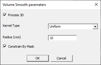
Computes a smoothed image by convolving the original image with a normalized
3D spherical (if 3D smoothing is selected) or circular (if 2D is selected) kernel,
or filter, with user-selected radius.
Creates a new layer with smoothed image.
Requires a 3D or 4D image, integer or real, in the active layer.
For a 4D (dynamic) dataset, each dynamic frame is smoothed independently.
May use an optional ROI to perform smoothing only within this ROI.
Once called, the command opens dialog to adjust the smoothing parameters
(Volume Smooth parameters, Fig. 15.1).
Process 3D (checkbox) – Selects spherical (3D, if checked)
or circular (2D, if unchecked) smoothing.
Kernel Type – Smoothing kernel options include: Uniform (default), Gaussian,
Radial, Raleigh, Median, Minimal SI, and Maximal SI.
Radius (vox) – Filter radius (in voxels).
Constrain by Mask (checkbox) – If checked, the visible ROI is used to perform
smoothing only within this ROI. If the document contains two or more visible ROIs,
this option is unavailable. To use it, uncheck visibility of all ROIs except one.
Example:
Consider a 2D uniform (kernel type: Uniform) smoothing using
a filter with the radius of 2 voxels. FireVoxel convention is to define a single
voxel as having the radius equal to 0. This means that the diameter of the circle
of radius 2 voxels is 5 voxels (diameter = 2 x radius + 1). The “circular” and
symmetric kernel with weights , is shown below:
In this example, the kernel has 13 non-zero weights. Since the kernel is uniform,
. All smoothing kernels are normalized, meaning that the sum
of 13 weights is 1.0. So in this example all weights are equal
to .
The smoothing operation works as follows. The kernel is positioned so that the central
element is above a target voxel. The values of 25 image voxels located
under this kernel are multiplied by the corresponding weights and
all products are summed. The resulting sum is the voxel value of the target voxel
in the smoothed image. The kernel is then moved to the next voxel and the process
is repeated until the entire smoothed image is computed.
For the uniform kernel, the weights are all equal, and as a result,
the smoothed voxel is the average of its 13 neighboring voxels.
For the Gaussian kernel, the weights are given by the values of
a Gaussian function.
Computes a smoothed dynamic image.
Requires a 4D image – integer, real, or 4D raster ROI.
Creates a new layer with the smoothed image.
Once called, the command opens dialog (Specify integer) to select
Dynamic Smooth Radius, or the number of dynamic frames over which
the intensity will be smoothed.
Smoothing is performed for each 3D coordinate (x,y,z) independently.
For the dynamic coordinate value N and user-selected dynamic smooth radius Rad,
the signal intensity values are averaged for all voxels within the dynamic
coordinate interval [N-Rad, N+Rad]. Void voxels are excluded from averaging.
If a voxel (x,y,z) at dynamic variable N is VOID, it remains VOID in
the smoothed image.
Computes a smoothed image within areas constrained by automatically
determined edges.
Requires a 3D or 4D image, integer or real, in the active layer.
For a 4D (dynamic) image, each dynamic frame is smoothed independently.
Creates a new, integer layer with the smoothed image.
Once called, the command opens dialog to adjust the smoothing parameters
(Edge-Constrained Smooth, Fig. 15.2):
If the image in the active layer is incompatible, shows an error message
(No suitable imag`present or enabled).
Creates a new layer with the smoothed image (real-valued, grayscale).
Once called, the command opens dialog (Edge-Constrained Smooth,
same as Fig. 15.2) to adjust the operation parameters.
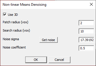
Computes a denoised image using a non-local means (NLM) filter.
Requires a 3D or 4D image, integer or real, in the active layer.
If the image is 4D (dynamic), applies denoising to each dynamic frame independently.
Creates a new layer with denoised image.
Once called, the command opens dialog (Non-local Means Denoising,
Fig. 15.3) to enter the parameters of the NLM filter.
This procedure is based on the most popular non-local means (NLM) denoising algorithm
[Buades2005]. The non-local means filter takes the mean of all voxels in the image
weighted by the similarity of these voxels’ neighborhood to the neighborhood of
the target voxel. FireVoxel extends the original 2D algorithm to 3D and makes it
fully parallel to gain speed.
Buades A, Coll B, Morel J-M. A non-local algorithm for image denoising.
Computer Vision and Pattern Recognition, 2005. Vol. 2. pp. 60–65.
doi:10.1109/CVPR.2005.38.
Parameters:
Use 3D – If checked, applies the 3D patch and searches over the entire volume.
Patch radius (vox) – The size (in voxels) of the spherical patch contained
within the specified (real) radius. Typically, the radius is in the [1,5] interval.
Note: Processing time grows roughly as radius^3 (radius cubed), and higher radius
values must be done judiciously.
Search radius (vox) – The size of the rectangular area where search and
accumulation of the similarity score is performed. Theoretically, this size
should be equal to the entire volume. However, since the execution time grows
roughly as the radius^3 (radius cubed), typically search radius=10 is used.
Higher or lower values may be used depending on the user’s hardware.
Noise sigma – A measure of the noise level. Controlled by the user to achieve
how strong denoising is.
Get Noise (button) – Calculates the Local Difference noise to give the user
an anchor value for operation.
Noise coefficient – Enables the choice between the two similar formulas
in the NLM implementation paper. Note: Build 373 – This parameter is currently
not used, but will be implemented in the future versions to allow access to
the second formula.
Requires a 3D or 4D image, integer or real. May also use an optional constraint ROI.
Creates a new layer with the edge map (real-valued, rainbow colormap by default).
When the command is selected:
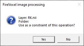
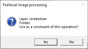
If the document contains a visible ROI layer, a dialog pops up:
If Yes is selected, then processing will be done only within this ROI.
If No is selected, then the entire image will be processed.
If the document contains two or more ROI layers, an error message is shown
(Ambiguous layer configuration).
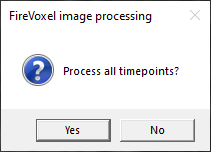
If the image is 4D, a dialog appears (Process all timepoints?):
If Yes is selected, each dynamic frame will be processed independently
and the result will also be a 4D image.
If No is selected, only the current frame will be processed, and
the result is 3D.
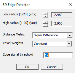
Next, the main dialog appears (3D Edge Detector, Fig. 15.4)
to adjust the parameters of edge detector. Processing starts once the user clicks OK.
The 3D Edge Detector dialog (Fig. 15.4) is used by
several commands, including Volume > Volume Edge-constrained smooth
and Inter-Volume Edge-constrained smooth, among others.
Low radius\High radius [1-20] (vox) – Lowest and highest size of features
calculated (in voxels). Default: 2.960 voxels.
Distance Metric – Calculation type for histogram comparison.
The options include Signal Difference or Histogram EMD (Earth Mover Distance).
Voxel Weights – Choice of voxel weights to account for the voxel distance
to the aperture center. The options include Constant, Gaussian, Radial,
and Rayleigh.
Edge signal threshold – Signal intensity threshold.
Calculates texture gradient for the user-selected single level of features
(characteristic size). This function uses an optional ROI (in which case
the analysis is performed only within this ROI) and also optionally processes
all timepoints in a 4D image. When the command is selected:
If a visible ROI is present, a question pops up:
If Yes is selected, the gradient map is calculated only within
the selected ROI. If No is selected, the gradient map is computed for
the entire image.
Next, if the original image is a 4D image, a dialog box pops up:
If Yes is selected, the operation is applied to all timepoints (each dynamic
frame is analyzed independently) and the resulting gradient map is also 4D.
If No is selected, the operation is applied only to the current timepoint
and the resulting gradient map is 3D.
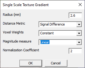
Next, the main dialog appears (Single Scale Texture Gradient,
Fig. 15.5) and processing starts once the user clicks OK.
Radius (mm) – Level (characteristic size, in millimeters) of the image
features calculated.
Distance Metric – Calculation type for histogram comparison.
The options include Signal Difference or Histogram EMD (Earth Mover Distance).
Voxel Weights – Choice of voxel weights to account for the voxel distance
to the aperture center. The options include Constant, Gaussian, Radial,
and Rayleigh.
Magnitude measure – Filter response value is converted to the output value
based on 3 different schemes: Linear, Logarithm, Normalized.
Normalization Coefficient – Coefficient used in Magnitude Measure=Normalize.
Calculates texture gradient for the range of feature levels and for each voxel
selects the maximum magnitude of the gradient. During segmentation, different
regions may be better separated at different feature levels, and therefore
an operation probing a range of feature levels may be able to separate these regions.
This function can also use an optional ROI and optionally process all timepoints.
When the command is selected:
If a visible ROI is present, a question pops up:
If Yes is selected, the resulting gradient map will be calculated only within
the selected ROI. If No is selected, the gradient is calculated over the entire
image.
Next, if the original image is a 4D image, a dialog box pops up:
If Yes is selected, the operation is applied to all timepoints (each dynamic
frame is analyzed independently) and the resulting gradient map is also 4D. If No is
selected, then the operation is applied only to the current timepoint (or dynamic frame)
and the resulting gradient map is 3D.
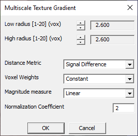
Next, the main dialog box appears (Multiscale Texture Gradient,
Fig. 15.6) and processing starts once the user clicks OK.
Low radius\High radius (vox) – Specifies the range of features calculated
(in voxels). Note the difference from the Single Scale Gradient radius, which is in mm.
Default: 2.6 voxels.
Distance Metric – Calculation type is Signal Difference or Histogram EMD
(Earth Mover Distance).
Voxel Weights – Choice of voxels weights to account for voxel distance to
the aperture center.
Magnitude Measure – Filter response value is converted to the output value based
on 3 different schemes: Linear, Logarithm, Normalized.
This function is similar to the regular multiscale texture gradient, but works only
for 4D Volumes. During a dynamic exam, the best separation between various pairs
of regions may be achieved at different timepoints. To take advantage of these optimal
separations, the function calculates the Multiscale Texture Gradient for each timepoint
separately. Then 4D Aggregate operation is performed, when for each voxel the maximum
gradient magnitude is selected across all timepoints and assigned to the resulting map.
Note that the result of this operation is always a 3D gradient map.
When the command is selected:
If a visible ROI is present, a question pops up:
If Yes is selected, the gradient map is calculated only within the ROI.
Next, the main dialog box appears (the same interface as for Multiscale Texture
Gradient, Fig. 15.6) and processing starts once the user clicks OK.
Parameters:
Low radius\High radius (vox) – Specify the lowest and highest size of features
calculated (in voxels). Note the difference to the Single Scale Gradient radius,
which is in mm. Default: 2.6 voxels.
Distance Metric – Calculation type includes Signal Difference or Histogram EMD
(Earth Mover Distance).
Voxel Weights – Choice of voxels weights to account for voxel distance to
the aperture center. The options include Constant, Gaussian, Radial, and Rayleigh.
Magnitude Measure – Filter response value is converted to the output value based
on 3 different schemes: Linear, Logarithm, Normalized.
Requires a 4D image with dimensions W x H x D x N, where W, H, and D are
width, height and depth, respectively, and N is the number of dynamic frames.
Creates a new document window named [active_window]_DtoT displaying the current
dynamic frame as W x H x 1 x D image. To scroll through slices, the user
may use Right and Left arrow keys on the keyboard.
If applied again to the W x H x 1 x D image, creates a new document window
displaying only the current slice (W x H x 1 x 1).
Requires a single slice across multiple dynamic points, W x H x 1 x N
(for other dimensions, shows an error message:
Volume should contain a single z-slice.)
Creates a new document window named [active_window]_TtoD with
reformatted image with dimensions W x H x N x 1. If used again on this new image,
shows an error message: 4D volume required.
Opens dialog (Specify Integer) to enter the target dynamic point index
where the current dynamic frame will be copied. Copies, voxel-by-voxel,
the current 3D dynamic frame onto the specified dynamic frame.
Requires a mosaic image (2D). Mosaic is a Siemens format for storing and displaying
a 3D image as a 2D, square array of slices shown as tiles from top left, row by row,
to bottom right.
If the original 3D image has voxel dimensions of W x H x D (in the column, row,
and slice directions, respectively), the dimensions of the mosaic image are
(p x W) x (p x H), where p is an integer ( rounded up
to the next integer). Thus, the mosaic is the smallest square array that
accommodates all slices of the original image.
Opens dialog (Specify Integer) to enter the number of images in the mosaic.
The default number of images is obtained from the private DICOM tag
0019,100A (Number of images in mosaic).
Transforms the mosaic into a regular 3D image with W x H x D dimensions.
Creates a new document window displaying the transformed image.
In a regular 3D image, the Columns tag is usually equal to the frequency columns value
in the Acquisition Matrix. For example, for a 3D image, the image dimensions tags may be
as follows:
0018,0093 Percent sampling 80
0018,1310 Acquisition Matrix 0\320\256\0
0028,0010 Rows 320
0028,0011 Columns 320
In a mosaic, the Acquisition Matrix tags indicate the dimensions of the individual images,
whereas the Rows and Columns tags contain the dimensions of the larger mosaic image,
equal to the multiples (p) of the dimensions of the individual images.
For example, for a 5 x 5 mosaic:
0018,1310 Acquisition Matrix 0\80\62\0
0028,0010 Rows 400
0028,0011 Samping 310
Note that these tags indicate the dimensions of the individual images and
the minimum dimensions of the square table required to accommodate this 3D image,
but not the total number of images.
Requires a visible real-valued image (in the active layer or another layer).
Opens dialog (Specify Integer) to enter the number of Resulting Bits
for integer-valued image (15 by default).
Creates a new layer in the active document window (named [original_layer]_integer)
with the original layer converted to integer-valued image.
The new layer is displayed with the same grayscale window width and level
as the original layer.
If the active layer is not a real-valued image and there are no other visible
real-valued layers, an error message is shown (Real valued volume is required).
If the active layer is not a real-valued image, but there are two or more visible
real-valued layers, the first visible layer (as listed in the Layer Control)
is converted.
Requires integer-valued image in the active layer.
Creates a new layer (named [original_layer]_real) containing the original layer
converted to a real-valued image.
If the active layer is not an integer-valued image, an error message is shown
(Signal intensity volume is required).
Requires a visible ROI layer.
Creates a new layer (named [original]_integer) with voxel values obtained from
the voxel values of the original layer converted to integer signal intensity.
The new layer is displayed as a rainbow colormap with the window width/level
of 1/0.5 and opacity of 100%.
If the active layer is not an ROI layer, and there is no visible ROI layer
in the document, the command shows an error message
(Signal intensity volume is required).
Requires a 3D integer image in the active layer.
Does not work for any other images. There are no parameters for this operation.
Creates a new layer in the same document window (named after as the original layer).
The distribution of intensities of the resulting image may be examined using
Layer Control > ROI Stats 3D.
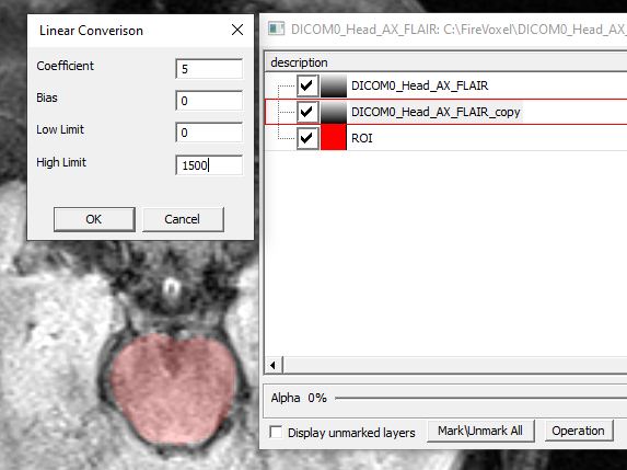
Linear conversion modifies voxel values of the original image.
Use Undo/Redo toolbar features if dissatisfied with results.
Keywords: scale, rescale, multiply, divide, normalize, ratio
Applies linear transformation to the image intensity values.
Requires an active image layer.
May also be used with a visible raster ROI layer.
If the document has a visible ROI, the transformation is applied only
within this ROI. If a visible ROI is not present, or if there are two
or more visible ROIs in the document, the conversion is applied to the entire image.
Opens dialog (Linear Conversion, Fig. 15.7)
to specify the parameters of linear conversion:
S1 = C x S0 + B,
where C is the coefficient, B is the bias, and converted S1 is
truncated within the user-specified signal interval [Low Limit, High Limit].
The operation replaces voxel intensities of the original image (S0)
with the transformed values (S1) within the ROI (if a visible ROI is present)
or within the entire image (if an ROI is not present).
The S1 values that fall below the Low Limit or above the High Limit
are replaced with the corresponding limit values.
Fig. 15.7 Voxel value linear conversion over ROI.
Example: Scale the image signal intensity within a selected area down by a factor of 7.
Draw an ROI manually over the selected area or use
segmentation tools such as EdgeWave Segmentation.
If the area contains only a few voxels, use Paintbrush and enter Radius of 0 voxels
in Paintbrush Properties to select individual voxels
one by one. Make sure that the ROI layer is visible.
Activate the image layer in Layer Control by clicking on its name.
Select Volume > Voxel value conversion > Linear conversion over ROI.
Enter Coefficient = 0.143 (= 1/7), Bias = 0, and appropriate Low and High Limit
values (Fig. 15.7). Click OK.
The intensity values within the ROI will be replaced with the scaled values.
If necessary, use Window and Level tool to adjust
the grayscale window for optimal viewing of the transformed values.
If dissatisfied with the result, use Undo function to revert
to the original state. Adjust the transformation parameters and repeat the operation
with these new parameters.
Invert modifies voxel values of the original image.
Use Undo/Redo toolbar features if dissatisfied with results.
For real and integer volumes: Replaces the original voxel intensities
S0 with symmetrical intensities about the middle of the interval
[S0min, S0max]. The distributions of the original and
inverted signal intensities can be examined using the histogram using
Layer Control > ROI Stats 3D.
For ROI layers: Changes the value of each voxel to the inverted value
(0<—>1): vnew = 1—v, where v and vnew are the old and
the new (inverted) voxel values, respectively.
Note: If you wish to modify only the appearance of the image
(rather than the image intensity values), use
Layer Control > View Filter
and check Invert Scale checkbox. This option inverts the display
of grayscale (the order of gray values) without changing the voxel values
in the volume.
Creates a new, real-valued layer in which voxel intensities
S1 are a log function of the original intensities
S0: S1= log(S0).
By default, the new layer is displayed as a rainbow color map.
Requires an image (integer or real) in the active layer.
Modifies voxel values of the original image.
The original voxel signal intensities S0
are replaced with transformed intensities S1.
Opens dialog (Specify Signal Range) to enter
[S1min, S1max], the minimum and maximum values
of the transformed intensity.
The original voxel intensities in the active layer, S0,
are replaced with transformed intensities
S1(x,y,z) = S1min + (S0(x,y,z) – S0min) x
(S1max – S1min)/(S0max – S0min).
Modifies voxel intensities of the original image.
Opens dialog (Specify Make Specified Signal Transparent)
to enter signal intensity value to be replaced with
a transparent voxel. Replaces voxels with user-specified intensities
with transparent voxels.
Requires an image in the active layer, presumably containing transparent voxels.
Modifies voxel intensities of the original image.
Opens dialog (Specify New value for transparent signal)
to enter the signal intensity value to be assigned to transparent voxels.
Replaces transparent voxels with opaque voxels with this user-specified
intensity value.
Opens dialog (Specify Uniform signal value) to specify
the signal intensity value.
Creates a new, real-valued layer with all voxels having this user-specified
intensity. The new layer is shown as a colormap and is placed on top of all existing
layers in the document.
Opens dialog (Specify string) to enter MRI sequence parameters.
Modality is not checked. The new values overwrite the original value
of the corresponding DICOM field.
Opens dialog (Specify string) to enter a sequence of four letters,
specifying the orientation of the volume with respect to the screen directions,
[Top, Bottom, Left, Right]. The letters should always form a 4-letter combination
without spaces or punctuation marks: SIRL, APLR, etc.
If the user enters implausible orientation, a warning will be displayed.
The allowed direction labels are: L — left, R — right, A — anterior,
P — posterior, S — superior, I — inferior.
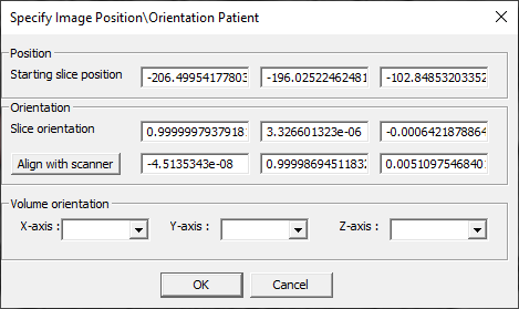
The Position and Orientation coordinates are read from DICOM header
fields ImagePositionPatient (20,0032) for starting slice and
ImageOrientationPatient (20,0037).
Clicking Align with scanner changes the orientation so that for each slice
the orientation axis is aligned with one of the scanner axes (1,0,0), (0,1,0),
or (0,0,1).
 .
.
 , is shown below:
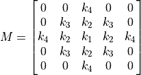
 . All smoothing kernels are normalized, meaning that the sum
of 13 weights is 1.0. So in this example all
. All smoothing kernels are normalized, meaning that the sum
of 13 weights is 1.0. So in this example all  weights are equal
to
weights are equal
to  .
. is above a target voxel. The values of 25 image voxels located
under this kernel are multiplied by the corresponding weights
is above a target voxel. The values of 25 image voxels located
under this kernel are multiplied by the corresponding weights 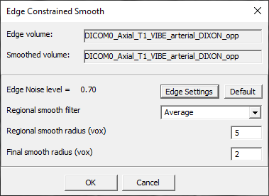
 rounded up
to the next integer). Thus, the mosaic is the smallest square array that
accommodates all slices of the original image.
rounded up
to the next integer). Thus, the mosaic is the smallest square array that
accommodates all slices of the original image.