29. Models
NOTE: May 11, 2022. Current FireVoxel Build 381.
This page is under construction. Content is added and edited daily.
The following models are available via Dynamic Analysis > Calculate Parametric Map in a dropdown menu labeled Model (see Fig. 28.1). Only models compatible with the current dataset are shown to the user. The compatible models are selected automatically based on the DICOM header information of the images in the current layer.
Signal measurements
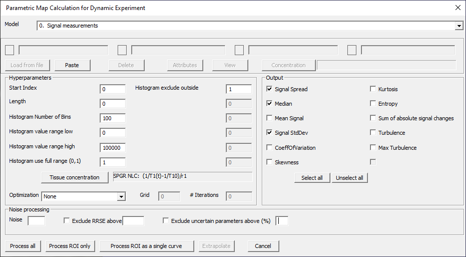
Fig. 29.1 Model 0.
Signal intensity
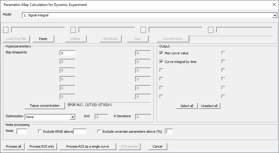
Fig. 29.2 Model 1.
Peak analysis
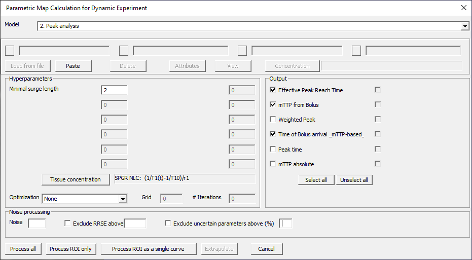
Fig. 29.3 Model 2.
Interleaved 2-state profile
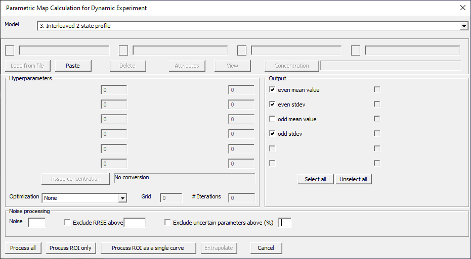
Fig. 29.4 Model 3.
Reference curve distance and correlation: 1IF
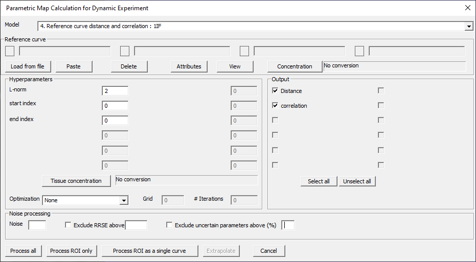
Fig. 29.5 Model 4.
Time of active rise
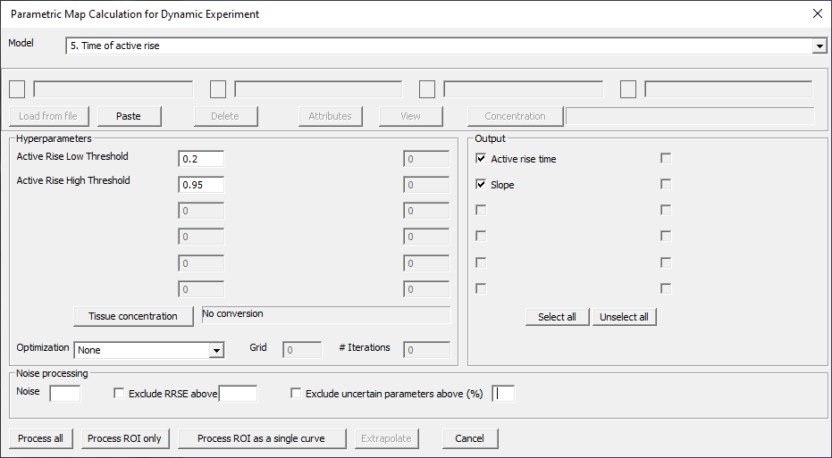
Fig. 29.6 Model 5.
Model 6
Model 7
Tofts two compartment exchange model {k-trans, Ve}: I1IF
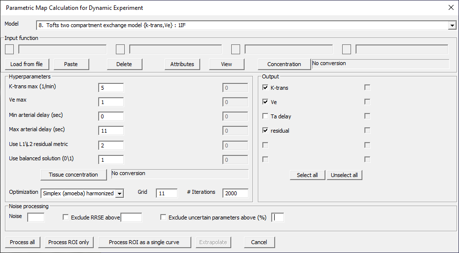
Fig. 29.7 Model 8.
Modified Tofts two compartment exchange model {k-trans, Ve, Va}: 1IF
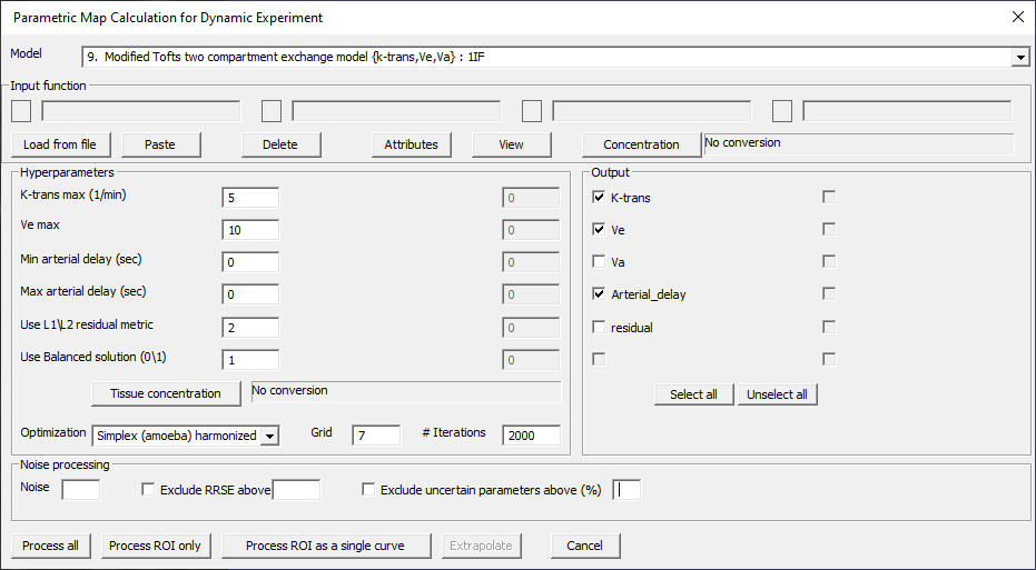
Fig. 29.8 Model 9.
RPF\vACx (AIF integration): 1IF
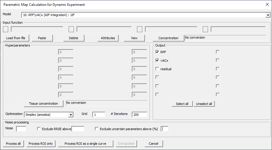
Fig. 29.9 Model 10.
RPF\vACx (AIF convolution): 1IF
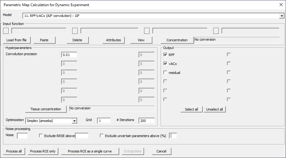
Fig. 29.10 Model 11.
Model 12
Transit Model {wa,ki,kti} (AIF convolution): 1IF
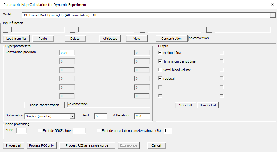
Fig. 29.11 Model 13.
GKM with two site water exchange: 1IF
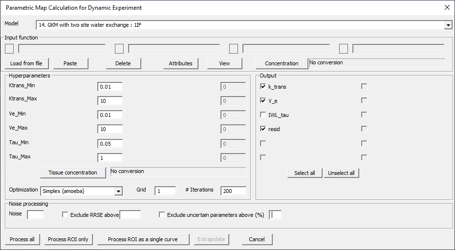
Fig. 29.12 Model 14.
Dual Input (Arterial\Portal Vein): {k_trans, V_e, Artf}: 2IF
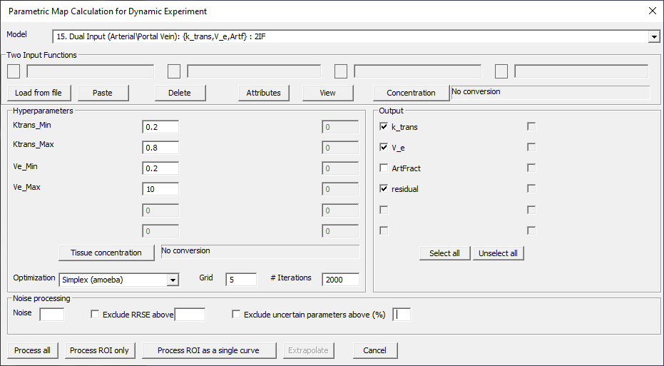
Fig. 29.13 Model 15.
16-21. Models 16-21
S = M0*(1-exp(-TD/T1)) with 6 fixed TD values
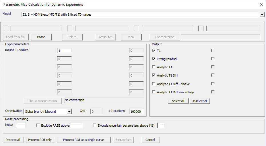
Fig. 29.14 Model 22.
S=M0*(1-exp(-TD/T1)) – 2 variables, TD=(700/4000) or TD=(350,700,1050,1750,2450,4000)
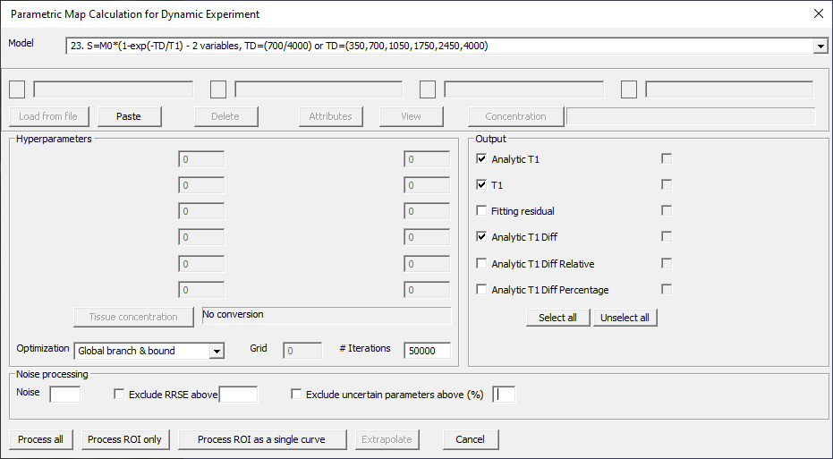
Fig. 29.15 Model 23.
24-42. Models 24-42
2CXM {vp,ve,Fp,PS} simplex optimization [Flouri 2016]: 1IF
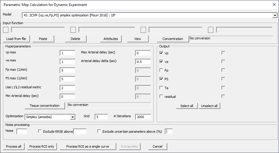
Fig. 29.16 Model 43.
Model 44
2CXM {vp,ve,Fp,PS} – LLS: 1IF
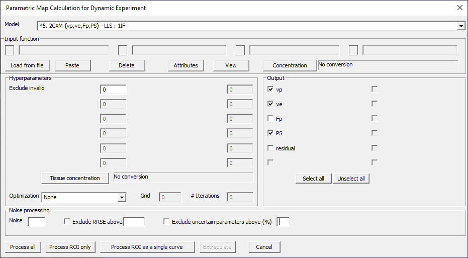
Fig. 29.17 Model 45.
Same as 43? 2CXM {vp,ve,Fp,PS} simplex optimization [Flouri 2016]: 1IF

Fig. 29.18 Model 46.
Tissue Uptake Model {vp,Fp,PS} simplex optimization [Sourbron 2013]: 1IF
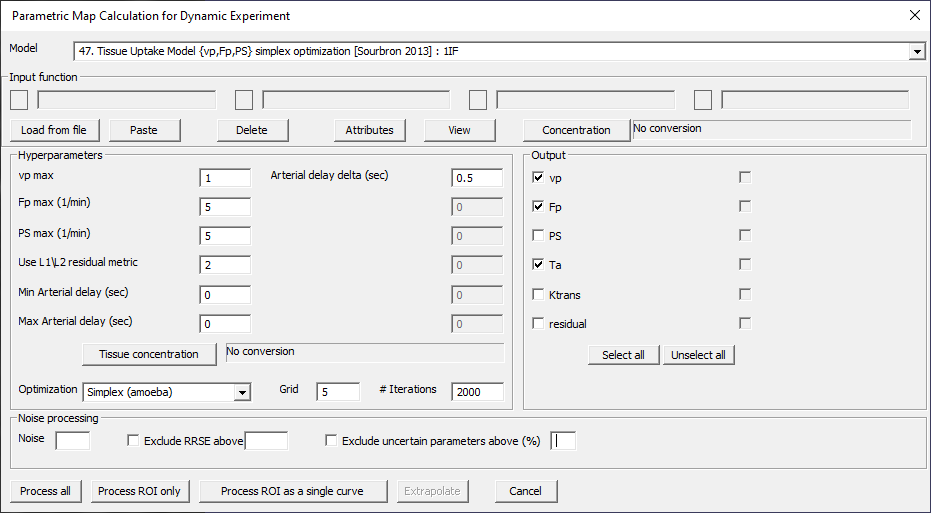
Fig. 29.19 Model 47.
Model 48
MR 2-Compartment Reference Region model [Yankeelov 2005]: 1IF
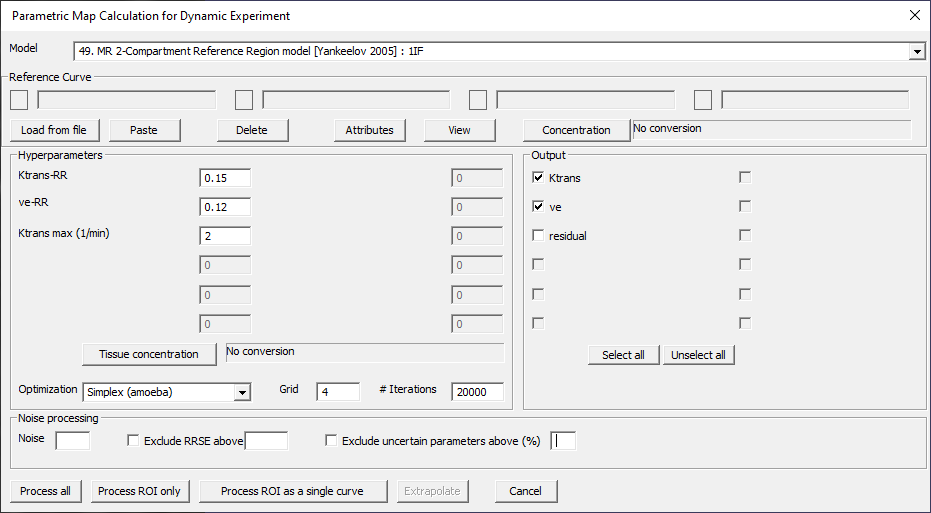
Fig. 29.20 Model 49.
Model 50
Model 51
Gamma Variate fit: Y(t) = K*((t-TA)/Tspan)^alpha*exp(-(t-TA)/Tspan/beta))
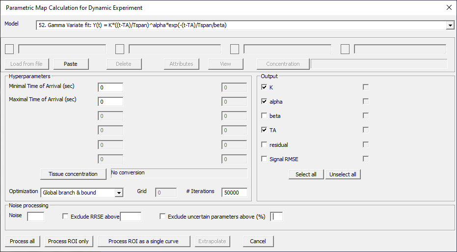
Fig. 29.21 Model 52.